Modelling Beyond a Straight Line

Detecting nonlinear and non-monotonic trends in water-quality monitoring data

1 Why I built this

I work in environmental consulting, where a lot of trend analysis still defaults to a straight line through the data because that’s what’s fast and familiar. Partway through a Master of Data Science, I started running into methods — piecewise regression, changepoint detection, GAMs — that would have changed how I read several records I’d already reported on, if I’d known them going in. This site is my attempt to connect those two sides: write up the methods the way I wish someone had explained them to me before I needed them, grounded in the kind of water-quality data an environmental consultant actually works with day to day.

As recommended by USEPA ProUCL for temporal trends, common practice is to use log-transformed ordinary least squares (OLS) to assess linearity, which I’ve worked through in a synthetic exercise in a separate repository here: https://github.com/iangault/vignette-temporal-trends.

2 Why nonlinear methods matter here

Environmental data rarely behaves as neatly as the models used to describe it. A straight-line trend is a fine description when a concentration is genuinely rising or falling at a constant rate — but many real records don’t look like that: a flat baseline that suddenly starts climbing, a level that jumps once and holds, a rise that levels off into a plateau, a seasonal cycle riding on top of a slower trend. Forcing a straight line onto any of these shapes produces a technically-fitted but practically misleading answer: it can make a plateaued analyte look like it’s still climbing, or smear a one-time step change into what reads as a gradual trend.

This site opens with two foundational chapters: a general regression framework for abstracting from raw data to a model - choosing a structure that actually matches the shape in front of you — (The Regression Framework), and a toolkit for diagnosing whether an apparent nonlinearity comes from the regressor or from the distribution of the response, and which transformation fixes it (Transformations). It then works through methods for detecting those same trajectories, in order of increasing flexibility — piecewise/segmented regression, changepoint detection, k-nearest-neighbors regression, LOESS smoothing, generalized additive models, and generalized additive mixed models for correlated residuals — plus a closing comparison of when the added flexibility is actually worth it against a plain linear fit.

3 What ordinary least squares is actually doing

Ordinary least squares models the conditional mean of the response given the regressors, not the response itself. For a single predictor:

\[y_i = \beta_0 + \beta_1 x_i + \varepsilon_i, \qquad \varepsilon_i \sim N(0, \sigma^2) \text{ i.i.d.} \qquad (1)\]

Equivalently, \(E[Y \mid X = x] = \beta_0 + \beta_1 x\) means that on average, at a given value of \(x\), expect this response value of \(y\) — a claim about the average trajectory, not any individual point.

The core assumptions, roughly in order of how much trouble breaking them causes:

Linearity — the true conditional mean really is a straight line in the predictors. This is the assumption every method on this site is about testing or relaxing.
Independence — residuals aren’t correlated with each other. Time-ordered data like these water-quality records are especially prone to violating this: a value close to the last one tends to stay close, producing autocorrelated residuals that standard OLS doesn’t account for (GAMM addresses this later).
Homoscedasticity — how far the observed response scatters around its fitted conditional mean is assumed to stay constant across the range of \(x\), not narrower at low values and wider at high ones (or vice versa).
Normality of errors — it’s the \(\varepsilon_i\) in equation (1) that’s assumed normal, not the response \(y_i\) itself. But since equation (1) defines \(y_i\) as \(\beta_0 + \beta_1 x_i\) plus \(\varepsilon_i\), a normal \(\varepsilon_i\) forces \(y_i\) to be normal too — just centered on \(\beta_0 + \beta_1 x_i\) instead of 0. What this assumption buys is valid \(t\)- and \(F\)-tests even at small sample sizes. Those tests work by comparing an estimate like \(\hat\beta_1\) against its sampling distribution — the distribution of values \(\hat\beta_1\) would take if the same study were repeated over and over on new samples — and that sampling distribution is only exactly normal when the underlying errors are exactly normal. At large sample sizes the Central Limit Theorem (CLT) — the result that a sum or average of many independent random quantities tends toward a normal distribution regardless of the shape of each one individually — makes the sampling distribution of \(\hat\beta_1\) approximately normal anyway, so the assumption matters most when the sample is small.

4 A model is an abstraction, not a recovery

Every method here — linear, piecewise, LOESS, GAM — is a different simplification of an unknown true process. The question is never which model is correct, it’s which simplification is adequate for the decision at hand and cheap enough to explain and defend. A straight line is a fine abstraction when the data really is monotonic; it becomes actively misleading once the shape genuinely bends.

5 Inference vs. prediction

Two different jobs a model can do, and every case study on this site is doing the first one:

Inference — the coefficients themselves are the answer: is there a real trend, how big is it, is it statistically distinguishable from noise. This requires the model form to be roughly right, since a misspecified model gives confident-looking, wrong numbers.
Prediction — only \(\hat y\) for new inputs matters; the model can be an uninterpretable black box as long as it’s accurate out-of-sample.

Not every method here can do inference, and that’s a structural property of the fitting procedure. For this site:

Inference-capable, and therefore prediction-capable too: linear regression, piecewise/segmented regression, changepoint detection, GAM, GAMM. Each produces an interpretable, testable parameter — a slope, a breakpoint location, a shift, a significance test on a smooth term — and the same fit gives a \(\hat y\) for free.
Prediction-only, structurally: k-nearest-neighbors and LOESS. Neither ever produces a coefficient or a p-value — there is no mechanism for one to come out of. What they supply is \(\hat y\) within the observed range of \(x\).

6 Types of models

Model choice is a tradeoff along three axes:

Interpretability — can the fitted model be explained to a non-statistician
Fit quality — does it capture the actual shape
Data efficiency — how much data it needs to estimate reliably

The methods on this site sit on a spectrum from parametric to nonparametric:

Parametric (linear, piecewise) — a small, fixed number of parameters. Highly interpretable and cheap to estimate, but correct only if the true shape matches the assumed form.
Nonparametric (k-nearest-neighbors, LOESS) — no fixed functional form; the fit adapts to local structure. Needs more data to estimate as reliably as a correctly-specified parametric model, and doesn’t reduce to a handful of reportable numbers.
Semi-parametric (GAM) — smooth basis functions like LOESS, but with a fitted penalty controlling how much wiggle is allowed, plus proper inferential machinery LOESS doesn’t provide.

7 Why this matters for a client or regulator

Model choice changes what gets reported and what action follows. A plateau misread as ongoing growth can trigger a treatment upgrade or permit renegotiation nobody actually needed. A step change misread as a gradual trend sends the investigation toward the wrong cause — a slow watershed process instead of the operational event or permit change that actually happened — and delays the fix. And a flexible model fit to pure noise manufactures a trend that isn’t there, triggering escalation over nothing. The reverse failure carries its own cost: real change dismissed as noise because the model wasn’t flexible enough to see it. Guarding against both means using the model whose complexity is actually supported by the data — no more, no less — and being able to explain that choice in plain terms to someone who isn’t a statistician, since a result nobody can sanity-check doesn’t get trusted enough to act on.

8 Start from the goal, not the method

The default reflex, faced with any time series, is to fit a straight line through it. That reflex is itself a form of model misspecification whenever the record isn’t actually a straight line. This site isn’t organized around one recommended method; it’s a set of starting points, one per goal, each demonstrated on a case study built to need it. The table below maps the goal to the chapter.

The Regression Framework and Transformations aren’t tied to any one row above — they’re the shared vocabulary and diagnostic checks every method in the table depends on.

What you’re trying to find out	Purpose	Definition	Start here	What you get
I just want to see the shape of the record before committing to any model form	Exploratory	Visualizing local structure with no fitted coefficients	k-Nearest Neighbors / LOESS	Prediction only, structurally — no coefficient or p-value comes out of either one
Is there a real trend at all, or would a flexible model just be fitting noise?	Diagnostic / triage	A general first check, not tied to one shape	Linear vs. Nonlinear Comparison	An inference answer: tested against “no added complexity is justified”
A permit change or effluent release may have shifted the slope — how do I quantify a break I can already see?	Confirmatory	Quantifying a break already visible in the record	Piecewise / Segmented Regression	Two slopes and a breakpoint location, each with a confidence interval
There may have been a spill that jumped the level to something new, and I don’t know when	Forensic	Locating an unknown event from the data alone	Changepoint Detection	A break location found by search, with a confidence interval and a significance test for whether a break exists at all
I have a large dataset with no single knot or known curve to fit, and I need a defensible significance test	General-purpose / flexible-but-inferential	Fitting a smooth curve without assuming its shape in advance	Generalized Additive Models	A smooth curve with an effective-degrees-of-freedom count and a significance test on the smooth term
The record is seasonal or regularly sampled, and residuals might not be independent (e.g. monthly monitoring)	Assumption check	Corrects a GAM’s result rather than posing a new goal	Generalized Additive Mixed Models	The same smooth-term test as a GAM, with standard errors that account for correlated residuals

A fitted model from any row above is typically a starting point of its own, not an endpoint — most chapters close with a short note on what a deeper analysis, built on top of what’s fitted there, would look like.

9 The case studies

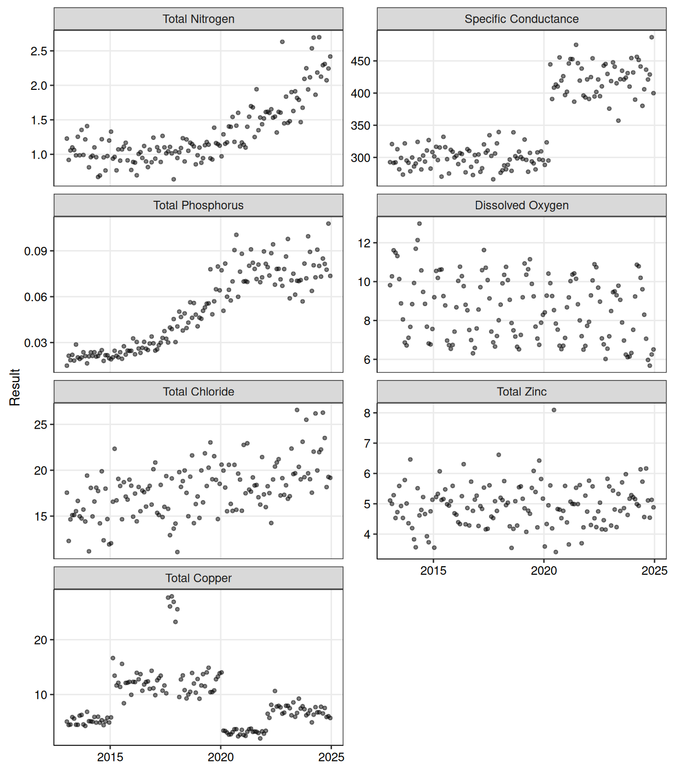
Seven analytes, each chosen to demonstrate a specific shape or to act as a control — monthly sampling, single composite site, 2013–2024.

Total Nitrogen — flat, then a genuine slope break. Piecewise/segmented regression: two slopes, one knot, no discontinuity.
Specific Conductance — a level jump at an unknown location. Changepoint detection: the same “something shifted” question as Total Nitrogen, but without being told where.
Total Phosphorus — a rise that levels into a plateau. Used twice — k-nearest-neighbors and LOESS, on the same data, for a direct side-by-side.
Dissolved Oxygen — a seasonal cycle riding on a longer-term trend, with residuals correlated month to month. GAMM: whether the trend’s significance survives once that correlation is modeled explicitly, rather than assumed away.
Total Chloride — a genuine, unremarkable straight-line trend. A control: the case where the simple linear model is already the right answer.
Total Zinc — pure noise, no real trend. The other control: the guard against a flexible model manufacturing a trend that isn’t there.
Total Copper — step-like and non-monotonic: up, up again into a brief spike, back down, further down, then a partial recovery. GAM: a shape with no periodic or polynomial pattern for a hand-built OLS feature to fall back on.

10 References

UBC Master of Data Science, DSCI 562: Regression II — Lecture 1: Link Functions and Count Regression, Lecture 6: Local Regression
Singh, A. and Singh, A.K. (2015). ProUCL Version 5.1 Technical Guide: Statistical Software for Environmental Applications for Data Sets with and without Nondetect Observations. EPA/600/R-07/041. U.S. Environmental Protection Agency, Office of Research and Development.