ggplot(control_wq, aes(year_frac, result)) +
  geom_point(alpha = 0.5) +
  geom_smooth(se = FALSE) +
  facet_wrap(~analyte, scales = "free_y") +
  labs(title = "Total Chloride and Total Zinc — raw scale", y = "Concentration") +
  nlt_theme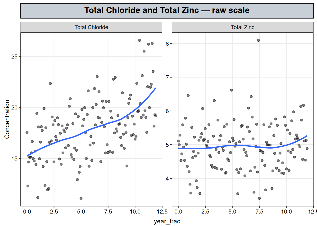
Total Chloride and Total Zinc — control cases
Every method chapter in this site handed a flexible term to a series that needed one: a hinge in piecewise regression, a level-shift indicator in changepoint detection, a smooth basis term in GAM — each an addition to the model’s systematic component, in the same sense The Regression Framework and GAM lay out. The choice each time was about matching the model’s flexibility to the complexity actually present in the series, not about reaching for the more sophisticated method on principle.
None of those chapters show what happens when that same flexibility is offered to a series that doesn’t need it. Getting the functional form right has real practical consequences: forcing unnecessary flexibility onto a series already well described by a straight line invites a model to report structure that isn’t there, and a client or regulator reading a wiggly fitted curve has no way to tell a genuine feature from an artifact of an over-flexible model. This section runs that check directly: a plain linear fit and a GAM, on the same data, for two analytes engineered to be control cases rather than case studies.
Total Chloride follows a real, unremarkable straight-line trend across the whole record — the case where a simple linear model is already the right answer, and a nonlinear model earns nothing extra for its added flexibility. Total Zinc has no real trend at all, just noise around a flat mean — the case where a flexible model could be tempted to fit that noise as if it were a shape. Concentration data is modeled on the log scale throughout this site, per Transformations; both analytes here follow that convention.
ggplot(control_wq, aes(year_frac, result)) +
geom_point(alpha = 0.5) +
geom_smooth(se = FALSE) +
facet_wrap(~analyte, scales = "free_y") +
labs(title = "Total Chloride and Total Zinc — raw scale", y = "Concentration") +
nlt_theme
Total Chloride climbs steadily with no visible bend; Total Zinc scatters around a flat level with no discernible pattern. Neither shape suggests a break, a plateau, or any structure a straight line wouldn’t capture.
For each analyte, lm(log(result) ~ year_frac) and mgcv::gam(log(result) ~ s(year_frac, bs = "tp", k = 20), method = "REML") are fit on the same data — the same GAM specification used in the GAM chapter, with the same k = 20 basis capacity, so the comparison isn’t handicapped by an artificially small smooth.
Two numbers do the actual comparing:
mgcv substitutes the smooth term’s edf, defined in GAM, for \(p\)) — lower is better, and the extra parameters a GAM’s smooth term is allowed to use only help its AIC if they buy enough of a likelihood improvement to outweigh their cost.summary(lm)$r.squared on the same log-scale response.fit_models <- function(sub) {
lin <- lm(log(result) ~ year_frac, data = sub)
gam_fit <- gam(log(result) ~ s(year_frac, bs = "tp", k = 20), data = sub, method = "REML")
list(lin = lin, gam = gam_fit)
}
chloride_wq <- control_wq |> filter(analyte == "Total Chloride")
zinc_wq <- control_wq |> filter(analyte == "Total Zinc")
fits_chloride <- fit_models(chloride_wq)
fits_zinc <- fit_models(zinc_wq)
comparison_table <- function(fits, label) {
s <- summary(fits$gam)
data.frame(
analyte = label,
model = c("Linear (lm)", "GAM"),
AIC = c(AIC(fits$lin), AIC(fits$gam)),
R2_or_dev_explained = c(summary(fits$lin)$r.squared, s$dev.expl),
smooth_edf = c(NA, s$edf),
smooth_p_value = c(NA, s$s.table[, 4])
)
}
rbind(
comparison_table(fits_chloride, "Total Chloride"),
comparison_table(fits_zinc, "Total Zinc")
) analyte model AIC R2_or_dev_explained smooth_edf
1 Total Chloride Linear (lm) -151.4800 0.287124636 NA
2 Total Chloride GAM -151.4797 0.287125180 1.000095
3 Total Zinc Linear (lm) -152.5135 0.006465102 NA
4 Total Zinc GAM -152.5132 0.006465640 1.000084
smooth_p_value
1 NA
2 0.0000000
3 NA
4 0.3380985Both analytes tell the same story: the smooth term’s effective degrees of freedom collapses to essentially 1 in both cases (edf ≈ 1.0) — the GAM’s own fitted penalty found no curvature worth keeping and shrank the smooth down to a straight line on its own, without being told the answer in advance. AIC is effectively tied between the two models for each analyte (the GAM’s slightly higher AIC reflects the small cost of estimating a penalty that ends up buying nothing), and the linear model’s \(R^2\) matches the GAM’s deviance explained almost exactly, because the two fits are, numerically, the same line.
The difference between the two analytes shows up in whether that line means anything. For Total Chloride, the smooth term is significant and deviance explained is substantial (28.7%) — a real trend, just a straight one. For Total Zinc, the smooth term is not statistically distinguishable from flat (\(p =\) 0.338) and deviance explained is negligible (0.6%) — there’s a line to draw through the noise, same as there would be through any random scatter, but nothing about the data supports treating it as a real trend.
grid_chloride <- data.frame(year_frac = seq(min(chloride_wq$year_frac), max(chloride_wq$year_frac), length.out = 200))
grid_zinc <- data.frame(year_frac = seq(min(zinc_wq$year_frac), max(zinc_wq$year_frac), length.out = 200))

build_grid <- function(grid, fits, label) {
  grid |>
    mutate(
      analyte = label,
      lin_fit = exp(predict(fits$lin, newdata = grid)),
      gam_fit = exp(predict(fits$gam, newdata = grid))
    )
}

fit_grid <- bind_rows(
  build_grid(grid_chloride, fits_chloride, "Total Chloride"),
  build_grid(grid_zinc, fits_zinc, "Total Zinc")
)

ggplot() +
  geom_point(data = control_wq, aes(year_frac, result), alpha = 0.35, color = "grey40") +
  geom_line(data = fit_grid, aes(year_frac, lin_fit, color = "Linear"), linewidth = 1) +
  geom_line(data = fit_grid, aes(year_frac, gam_fit, color = "GAM"), linewidth = 1, linetype = "dashed") +
  facet_wrap(~analyte, scales = "free_y") +
  scale_color_manual(values = c(Linear = "steelblue", GAM = "#A85751"), name = NULL) +
  labs(title = "Total Chloride and Total Zinc — linear vs. GAM fit", y = "Concentration") +
  nlt_theme +
  theme(legend.position = "right")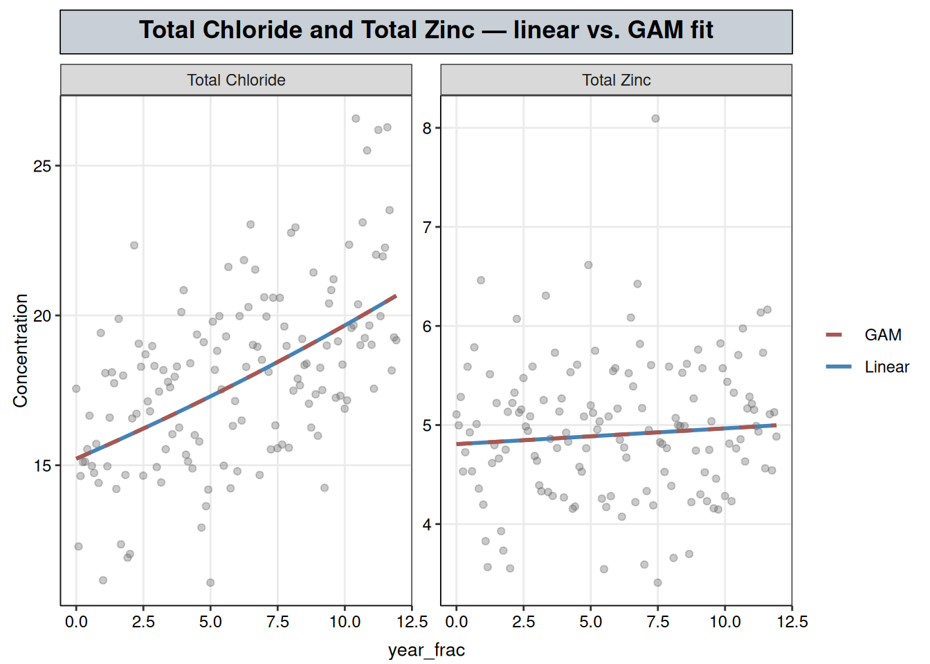
The dashed GAM line sits almost exactly on top of the solid linear line in both panels — visual confirmation of the edf ≈ 1 result above. The GAM was free to bend and chose not to, in both directions: it didn’t flatten Total Chloride’s real trend, and it didn’t manufacture curvature out of Total Zinc’s noise.
bptest(fits_chloride$lin)
    studentized Breusch-Pagan test

data:  fits_chloride$lin
BP = 0.78299, df = 1, p-value = 0.3762shapiro.test(resid(fits_chloride$lin))
    Shapiro-Wilk normality test

data:  resid(fits_chloride$lin)
W = 0.99208, p-value = 0.604bptest(fits_zinc$lin)
    studentized Breusch-Pagan test

data:  fits_zinc$lin
BP = 0.073089, df = 1, p-value = 0.7869shapiro.test(resid(fits_zinc$lin))
    Shapiro-Wilk normality test

data:  resid(fits_zinc$lin)
W = 0.98644, p-value = 0.1702
Both linear fits pass both tests: Total Chloride shows no heteroscedasticity (\(p = 0.376\)) and no non-normality (\(p = 0.604\)); Total Zinc likewise shows no heteroscedasticity (\(p = 0.787\)) and no non-normality (\(p = 0.170\)).
Box.test(resid(fits_chloride$lin), lag = 1, type = "Ljung-Box")
    Box-Ljung test

data:  resid(fits_chloride$lin)
X-squared = 0.24523, df = 1, p-value = 0.6205Box.test(resid(fits_zinc$lin), lag = 1, type = "Ljung-Box")
    Box-Ljung test

data:  resid(fits_zinc$lin)
X-squared = 0.50219, df = 1, p-value = 0.4785
Both also pass the independence check: Total Chloride (\(p = 0.621\)) and Total Zinc (\(p = 0.479\)) both show no evidence of residual autocorrelation. Nothing in either fit’s residuals argues against treating the linear model as adequate for either analyte.
Neither control case rewards the extra flexibility a GAM offers, and the simple linear model is the right one to report for both. On Total Chloride, the GAM’s fitted penalty reproduces the linear trend almost exactly, at the cost of a slightly worse AIC for buying flexibility that goes unused — the straight line already captures the real trend in the data. On Total Zinc, a flexible model, free to bend, chose not to: the flat line isn’t hiding a suppressed trend the smoother could have caught, it’s simply the right description of noise around a constant mean. That’s the practical value of this comparison for a client or regulator report — model choice should be no more flexible than the data actually supports, and the extra machinery of a GAM, a piecewise fit, or a changepoint model is worth reaching for only when a series’ shape actually calls for it, as the earlier chapters’ case studies did.
This chapter ran the lm-vs-GAM comparison on two analytes chosen in advance to explore lm()-vs-gam()-by-AIC comparison for any series where a plot leaves real doubt about whether a bend is genuine or just noise. It isn’t a step every series needs: for most analytes, the raw plot already settles the question — a visibly straight trend or a visibly flat scatter doesn’t need a fitted GAM to confirm what’s apparent by eye. This chapter is for the narrower case where that visual judgment is genuinely unclear and a fitted comparison is worth the effort to settle it.