The Regression Framework
Where ordinary least squares sits, and what each method on this site changes about it
1 A model has five moving parts
In plain terms, every regression model is just a formal way of saying “the response’s typical value depends on the regressor, plus some leftover noise around that typical value.” Everything below is about pinning down that sentence precisely enough to fit: what “typical value” means, how the noise behaves, what shape the dependence takes, and how the numbers get estimated.
The reason to bother getting each of those five parts right, rather than just eyeballing a curve through the points, is that a correctly specified model is what turns a fitted line into a defensible statistical claim — a confidence interval, a p-value, a statement that a trend is real and not noise.
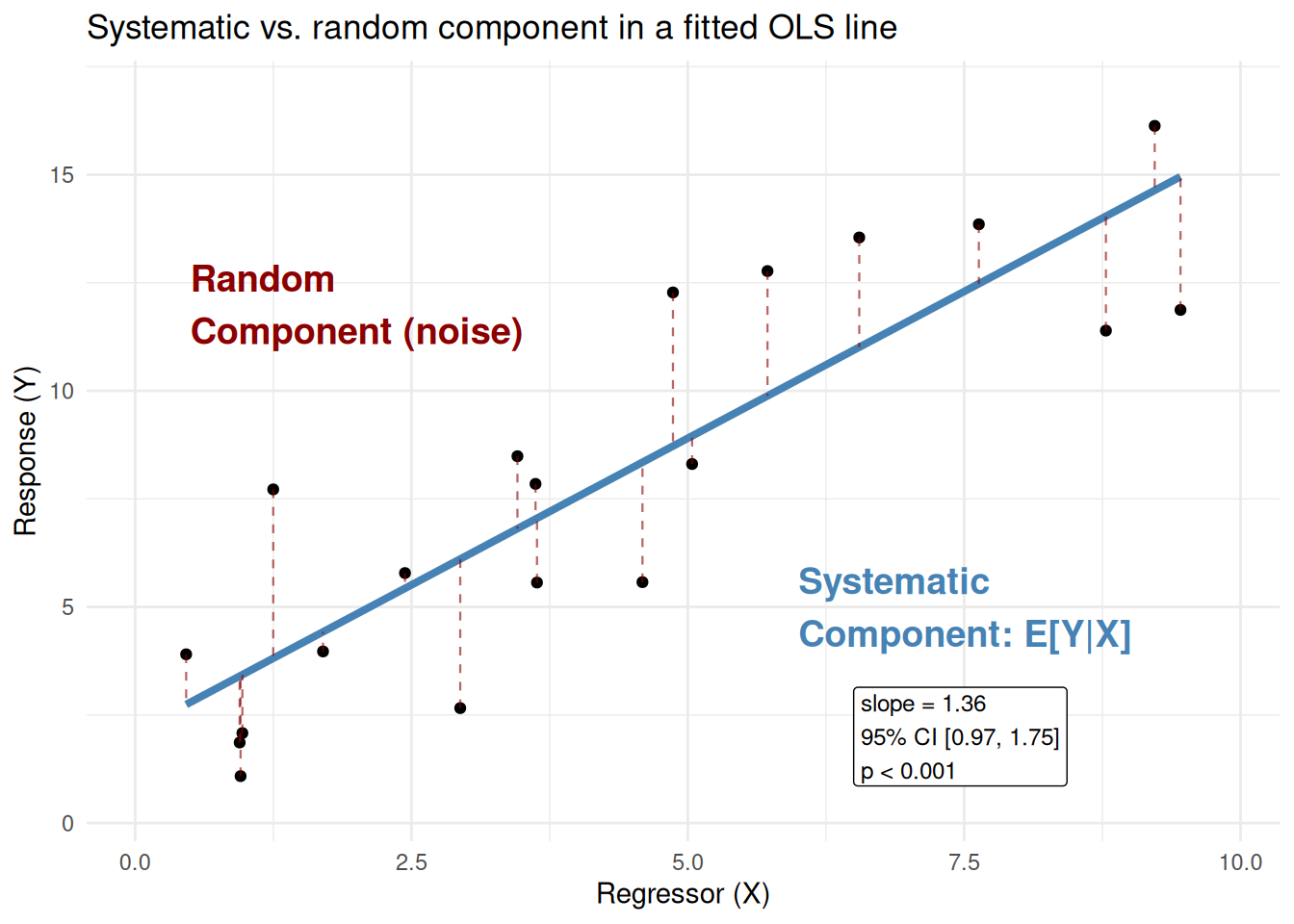
The figure below is a simple linear fit, lm(y ~ x), i.e. \(y_i = \beta_0 + \beta_1 x_i + \varepsilon_i\):
The fitted line is the systematic component, \(E[Y \mid X]\); the vertical gap between a point and the line is the random component for that observation. Getting both right — the shape of the line and the behavior of the scatter around it — is what supports the inference step later.
1.1 Data Modelling Framework
Conceptually, the OLS regression model can be expressed as:
\[ \mbox{Response} = \mbox{Systematic Component} + \mbox{Random Component}. \tag{1}\]
- The systematic component represents the mean of the response, conditioned on the regressor values.
- The random component measures the extent to which the observed value of the response might deviate from its mean.
For the \(i\)th observation in our random sample or training data (\(i = 1, \dots, n\)), the conceptual model, from Equation 1, is mathematically represented as:
\[ \underbrace{Y_i}_\text{Response} = \underbrace{\beta_0 + \beta_1 g_1(X_{i, 1}) + \ldots + \beta_k g_k(X_{i,k})}_\text{Systematic Component} + \underbrace{\varepsilon_i.}_\text{Random Component} \tag{2}\]
Note the following:
- The response \(Y_i\) is equal to the sum of \(k + 2\) terms on the right-hand side.
- The systematic component is the sum of:
- An unknown intercept \(\beta_0\) and
- \(k\) regressor functions \(g_j(X_{i,j})\) (\(j = 1, \dots, k\)) multiplied by their respective unknown regression coefficient \(\beta_j\).
- \(\varepsilon_i\) is the random noise for the \(i\)th observation.
Modelling Assumptions
The model in Equation 2 above for \(Y_i\) is more detailed as follows:
The response \(Y_i\) depends on the linear combination of the functions \(g_j(\cdot)\) of \(k\) regressors \(X_{i, j}\) of different types (continuous and discrete).
Each function \(g_j(X_{i,j})\) has an associated regression coefficient. These parameters \(\beta_{1}, \dots, \beta_{k}\) represent how much the response is expected to increase or decrease when the function \(g_j(X_{i,j})\) changes by one unit of the \(j\)th regressor. An additional parameter, \(\beta_0\), represents the mean of the response when all the \(k\) functions \(g_j(X_{i,j})\) are equal to zero. All these elements represent the systematic component of the model.
The term \(\varepsilon_i\) is an unobserved random variable representing the random component. These variables are assumed to be normally distributed with mean zero and a common variance \(\sigma^2\) — homoscedasticity — and independent of each other.
TipDefinition of random component assumptions in OLS
\[ \begin{gather*} \mathbb{E}(\varepsilon_i) = 0 \\ \text{Var}(\varepsilon_i) = \sigma^2 \\ \varepsilon_i \sim \mathcal{N}(0, \sigma^2) \\ \varepsilon_i \perp \!\!\! \perp \varepsilon_\ell \; \; \; \; \text{for} \; i \neq \ell \; \; \; \; \text{(independence)}. \end{gather*} \]
1.2 The five parts
Fitting a regression model means making five separate choices, whether or not they’re stated explicitly:
- Estimand — what aspect of \(Y \mid X\) is actually being modeled. Ordinary least squares targets the conditional mean, \(E[Y \mid X]\). A model could instead target the median or a quantile; that choice determines everything downstream.
- Random component — how \(Y\) scatters around that estimand. OLS assumes \(Y_i \mid X_i \sim N(\mu_i, \sigma^2)\): Gaussian noise, the same variance at every value of \(X\).
- Link function — the function connecting the mean to the linear predictor, \(g(\mu_i) = \eta_i\). OLS uses the identity link, \(g(\mu) = \mu\), whose transformation is trivial enough that OLS is easy to mistake for having no link function at all.
- Systematic component — how the regressors combine into the linear predictor, \(\eta_i = \beta_0 + \beta_1 X_{1i} + \beta_2 X_{2i} + \cdots\).
- Estimation — the numerical values of the \(\beta\)’s that fit the data. OLS minimizes the sum of squared residuals; under the Gaussian assumption in step 2, that’s identical to maximum likelihood.
1.3 OLS as one specific setting
Ordinary least squares is one specific setting of all five parts: conditional mean, Gaussian noise, identity link, a linear-in-the-parameters systematic component, least squares. Every other method on this site changes one of those five slots relative to OLS — but the methods aren’t siblings that each pick a different slot independently. They nest: GLM ⊆ GAM ⊆ GAMM, where each one can do everything the one before it could, plus one more thing.
- A generalized linear model changes the link and/or the random component — a log link, Poisson or Gamma noise — while keeping the systematic component linear in \(\beta\). Setting the link to identity and the noise to Gaussian reduces a GLM to OLS.
- A generalized additive model (see Generalized Additive Models) keeps everything a GLM has — it can still use a log link, Poisson noise, whatever the data calls for — and additionally lets the systematic component itself be a smooth function, \(\beta_0 + f(X)\), estimated from the data, instead of forcing \(\beta_0 + \beta_1 X\). Restricting \(f(X)\) to a straight line reduces a GAM to a GLM.
- A generalized additive mixed model (see Generalized Additive Mixed Models) keeps everything a GAM has — link, noise family, smooth terms — and additionally lets the random component’s independence assumption go, allowing correlated residuals. Dropping that correlation structure reduces a GAMM to a GAM.
1.4 What later chapters change
Framed this way, none of the methods on this site is a full departure from OLS. Each one relaxes exactly one of the five assumptions above, in a specific, nameable way, while leaving the rest of the framework intact.
2 “Linear” means linear in the coefficients, not straight in \(X\)
A regression is a linear model if the systematic component is a linear combination of terms — linear in the \(\beta\)’s — regardless of whether those terms are linear functions of the original regressor.
For example, lm(y ~ x + I(x^2)) fits:
\[y_i = \beta_0 + \beta_1 x_i + \beta_2 x_i^2 + \varepsilon_i,\]
Where I() (“as-is”) tells R to evaluate x^2 as literal arithmetic and use the result as a predictor column, overriding the formula operator’s usual special meaning.
This produces a curved fitted line in \(x\) while remaining a linear model: the fit is still a linear combination of the columns \(\{1, x, x^2\}\), estimated the same way a simple straight line would be.
As another example, piecewise-regression.qmd uses the same trick with a hinge term instead of a squared term — \(\beta_2 (x_i - c)_+\), where \((x - c)_+ = \max(0, x - c)\) is zero for \(x \le c\) and equal to \(x - c\) for \(x > c\) — a column that’s flat before the breakpoint \(c\) and ramps up linearly after it, letting the slope change at \(c\) without a break in the fitted line. It’s one more column handed to lm(), not a different kind of model.
In addition, feature-engineering the regressor bends the fitted curve without ever leaving step 4 of the framework above (linear combination of \(\beta\)’s); it’s a different move from transforming the response or changing the link, which will be explored more in Transformations.
3 Multiple regressors, and why visualizability breaks down the way it does
A single continuous regressor gives a fit that’s a line or curve in two dimensions — fully visualizable. Two continuous regressors give a fit that’s a surface in three dimensions — still visualizable, if harder to draw by hand. Three or more continuous regressors give a fit with no direct picture at all; it’s still “linear in the \(\beta\)’s,” it just can’t be drawn.
A categorical regressor produces a family of lines within the same 2D picture, one per category, either parallel (an additive model) or free to diverge (an interaction model) — rather than adding a dimension the way a second continuous regressor would. This project only ever has one regressor — time — so that distinction is never exercised in the case studies here; it matters for reading models elsewhere, such as the year-by-monitoring-area trend models in the sibling vignette-temporal-trends project, where “area” is exactly this kind of categorical regressor.
4 A different estimand: ProUCL’s UCLs vs. this site’s trend models
EPA’s ProUCL software is the standard tool for computing environmental decision statistics — Upper Confidence Limits, Upper Tolerance Limits, background threshold values, exposure point concentrations — and worth placing against the five-part framework above, since it targets a different estimand than every method on this site. ProUCL’s core statistics summarize a single, time-collapsed sample into one population parameter (a bound on a fixed mean or percentile), not a conditional mean \(E[Y \mid X]\) estimated as a function of a regressor. That mismatch in estimand — step 1 of the five parts — is why ProUCL’s well-known Gamma-vs-lognormal distribution choice for those statistics has no direct analog here: it answers “what is the population mean,” not “how does the mean change with \(X\).”
Where ProUCL does share this site’s estimand is its separate Trend Analysis module, which fits OLS as a function of time and pairs it with the nonparametric Mann-Kendall and Theil-Sen tests as a cross-check — the same conditional-mean target, the same parametric/nonparametric pairing used in this site’s case studies and worked through directly in the companion vignette-temporal-trends project. Transformations covers this distinction, and where ProUCL’s transformation-bias caution does and doesn’t apply, in more depth.
5 What comes next
The rest of this site works through methods in order of increasing flexibility, and most of them still fit inside the five-part framework above, each changing exactly one slot: a hinge term on the regressor (piecewise regression), a mean shift at an unknown location (changepoint detection), a flexible smooth term with proper inference (GAM), and an explicit model for correlated residuals (GAMM).
k-nearest-neighbors and LOESS are the exception to this pattern: neither has a systematic component that’s linear in any coefficients. That absence of inherited structure is exactly what makes them useful as a fully nonparametric baseline.
Transformations, next, covers the response-side and regressor-side tools available before reaching for any of them — and how to tell which one a given series actually needs.