ggplot(tn, aes(year_frac, log(result))) +
  geom_point(alpha = 0.5) +
  geom_smooth(se = FALSE) +
  labs(title = "Total Nitrogen — log scale") +
  nlt_theme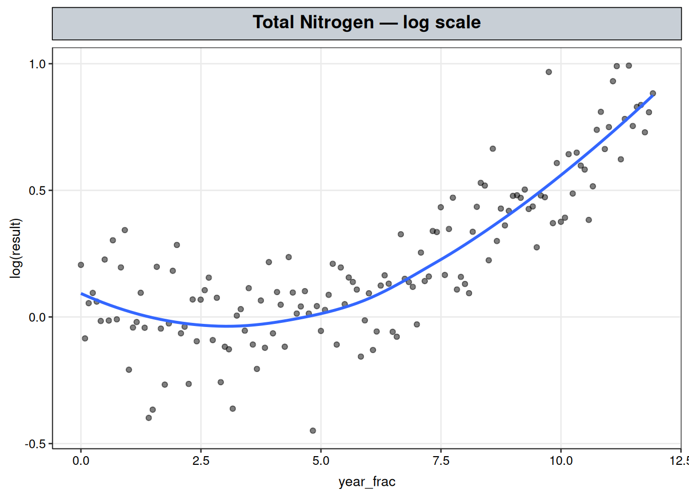
Total Nitrogen — a genuine break in slope
A straight-line regression assumes one slope holds across the whole record. Three progressively less restrictive models relax that assumption:
Total Nitrogen — flat, then a genuine slope break, with no discontinuity in level — belongs at the third stage: two slopes joined at a single knot.
A hinge function is feature engineering on the regressor rather than a link function — see The Regression Framework for why a model with a hinge term is still fit by lm(), and how that differs from a link function.
log(result)Concentration data is fit on the log scale throughout this site: it matches the multiplicative-process story concentration data tends to follow, and it corrects the variance-growing-with-the-mean residual pattern (a distributional problem, in the Breusch-Pagan/Shapiro-Wilk sense) that fitting the raw scale directly would leave behind — both covered in Transformations.
A consequence: the hinge-term coefficient \(\hat\beta\) comes out of the model in log-units per year, not concentration units, so it isn’t itself a usable rate. Back-transforming it, \((\exp(\hat\beta) - 1) \times 100\%\), converts that log-scale slope into a constant percentage rate of change — the number actually reported for the post-break segment below.
ggplot(tn, aes(year_frac, log(result))) +
geom_point(alpha = 0.5) +
geom_smooth(se = FALSE) +
labs(title = "Total Nitrogen — log scale") +
nlt_theme
Although the breakpoint is known from the syntheic data, it was not assumed to be known in our analysis: it was estimated from the data using segmented::segmented(), seeded from an initial visual read of the series.
That function starts from a baseline model with a single global slope and no breakpoint, then runs an iterative local search — Muggeo’s algorithm: re-estimate the breakpoint given the current slopes, re-estimate the slopes given the new breakpoint, repeat to convergence — around the starting value. It is a local search rather than an exhaustive one, so the starting value needs to be in the right neighborhood rather than exact; here, roughly year 6 (psu = 6) into the twelve-year record, read off the plot above.
lm_tn <- lm(log(result) ~ year_frac, data = tn)
seg_tn <- segmented(lm_tn, seg.Z = ~year_frac, psi = 6)NAsummary(seg_tn)
    ***Regression Model with Segmented Relationship(s)***

Call:
segmented.lm(obj = lm_tn, seg.Z = ~year_frac, psi = 6)

Estimated Break-Point(s):
                 Est. St.Err
psi1.year_frac 5.892  0.361

Coefficients of the linear terms:
              Estimate Std. Error t value Pr(>|t|)
(Intercept)   0.010125   0.035902   0.282    0.778
year_frac    -0.001482   0.010630  -0.139    0.889
U1.year_frac  0.141293   0.014729   9.593       NA

Residual standard error: 0.153 on 140 degrees of freedom
Multiple R-Squared: 0.7655,  Adjusted R-squared: 0.7604

Boot restarting based on 6 samples. Last fit:
Convergence attained in 2 iterations (rel. change 9.5288e-13)
The coefficient table above reports Pr(>|t|) as NA for the change-in-slope term, U1.year_frac. That’s expected rather than missing. A standard \(t\)-test on a regression coefficient assumes the design matrix — the columns of regressor values lm() is fed — is fixed, known in advance, not something estimated from the same data the coefficient is fit on. Here it isn’t fixed: U1.year_frac’s column is \((x_i - \hat c)_+\), built from the estimated breakpoint \(\hat c\), so the regressor a reader would need held fixed to trust the usual \(t\)-distribution was itself derived from this dataset’s outcomes.
That breaks the assumption the reference distribution relies on, so segmented reports NA rather than a number that would overstate precision. confint() and slope() below are the package’s alternative — inference on the breakpoint and on each segment’s slope that accounts for \(\hat c\) being estimated rather than given.
confint(seg_tn) Est. CI(95%).low CI(95%).up
psi1.year_frac 5.89162 5.17792 6.60531slope(seg_tn)$year_frac
Est. St.Err. t value CI(95%).l CI(95%).u
slope1 -0.0014823 0.010630 -0.13944 -0.022499 0.019534
slope2 0.1398100 0.010196 13.71300 0.119650 0.159970The breakpoint is estimated at year_frac ≈ 5.9 (95% CI 5.18–6.61) — roughly 5.9 years into the twelve-year record. Before the break, there is no detectable trend over the first six years. After the break, the slope is clearly positive (95% CI 0.120–0.160, i.e., excluding zero); back-transformed, \((\exp(0.140) - 1) \times 100\% \approx 15\%\) per year.
slope()’s output reports a \(t\)-value but no p-value, for the same reason as the NA above — the reference distribution for that statistic isn’t exact once the breakpoint is estimated rather than fixed. The confidence interval carries the same caveat but is what the package leads with, rather than a p-value that would look more precise than the estimation actually supports. It doesn’t change the reading: the interval excludes zero for the post-break slope and includes it for the pre-break slope, the same conclusion a p-value would give.
tn_pred <- tn |> mutate(fitted = predict(seg_tn))

slope2 <- slope(seg_tn)$year_frac["slope2", ]
slope2_label <- sprintf(
  "slope 2 = %.3f (95%% CI %.3f-%.3f)",
  slope2["Est."], slope2["CI(95%).l"], slope2["CI(95%).u"]
)

ggplot(tn, aes(year_frac, log(result))) +
  geom_point(alpha = 0.5) +
  geom_line(data = tn_pred, aes(y = fitted), color = "steelblue", linewidth = 1) +
  geom_vline(xintercept = seg_tn$psi[, "Est."], linetype = "dashed") +
  annotate(
    "label",
    x = seg_tn$psi[, "Est."] + 0.2, y = max(log(tn$result)),
    label = slope2_label, hjust = 0, vjust = 1, size = 3.2
  ) +
  labs(title = "Total Nitrogen — continuous piecewise fit (log scale)") +
  nlt_theme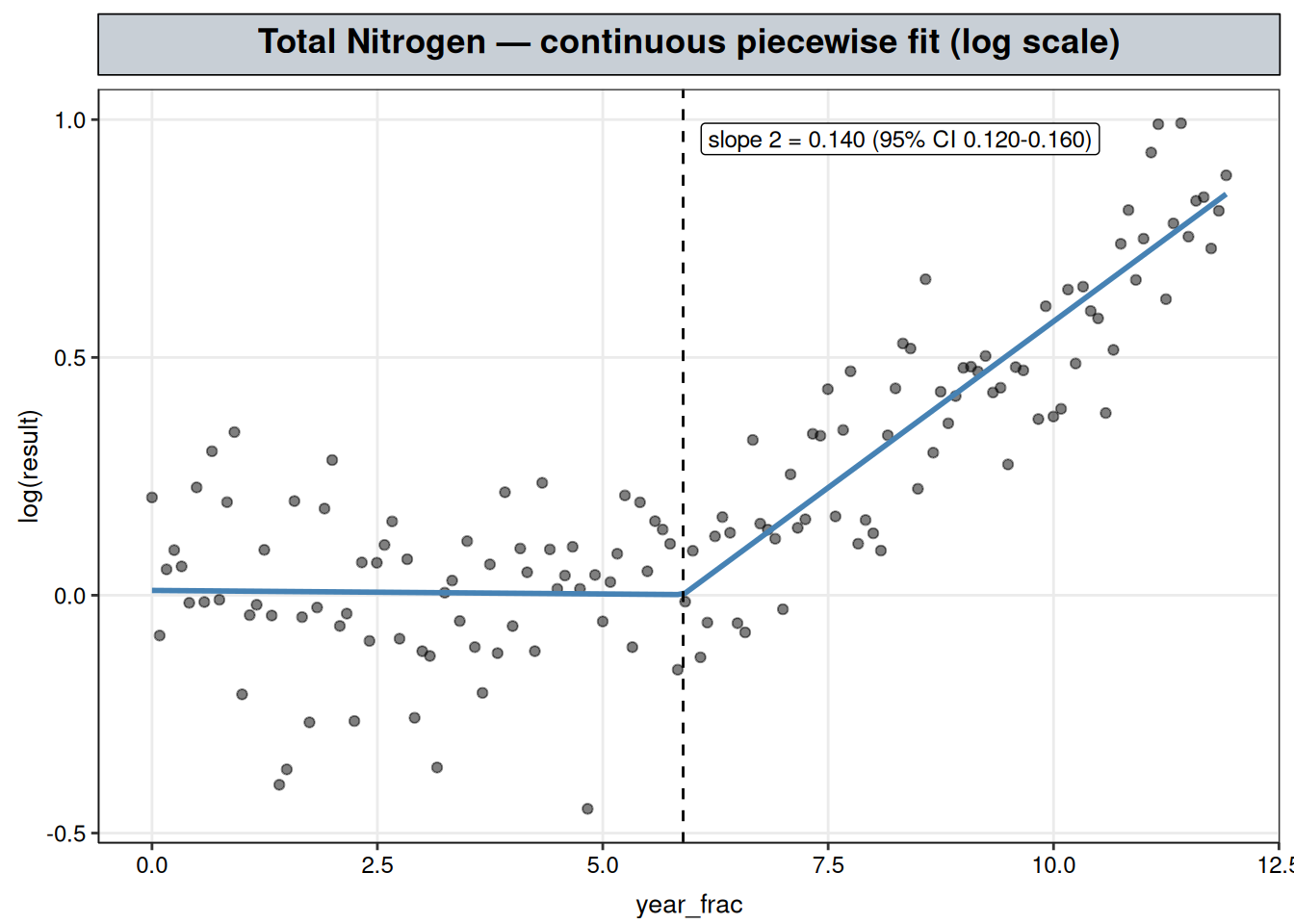
The segmented fit carries the same ordinary-least-squares assumptions as the underlying linear model — homoscedasticity and normally distributed residuals (see Transformations for why these checks matter and what they do and don’t catch).
bptest(seg_tn)
    studentized Breusch-Pagan test

data:  seg_tn
BP = 3.4454, df = 3, p-value = 0.3279shapiro.test(resid(seg_tn))
    Shapiro-Wilk normality test

data:  resid(seg_tn)
W = 0.99181, p-value = 0.575
Both tests fail to reject their null: the Breusch-Pagan test (\(p = 0.328\)) finds no evidence of heteroscedasticity, and the Shapiro-Wilk test (\(p = 0.575\)) finds no evidence of non-normal residuals. This is also a retroactive check on the log-transform: a failure in either test would have suggested log(result) wasn’t the right scale to model on.
A third assumption — independence — isn’t covered by either test above, and monthly monitoring data has an obvious way to violate it: this month’s reading sitting closer to last month’s than an independent draw would. Checked directly:
acf(resid(seg_tn), main = "Total Nitrogen — residual autocorrelation")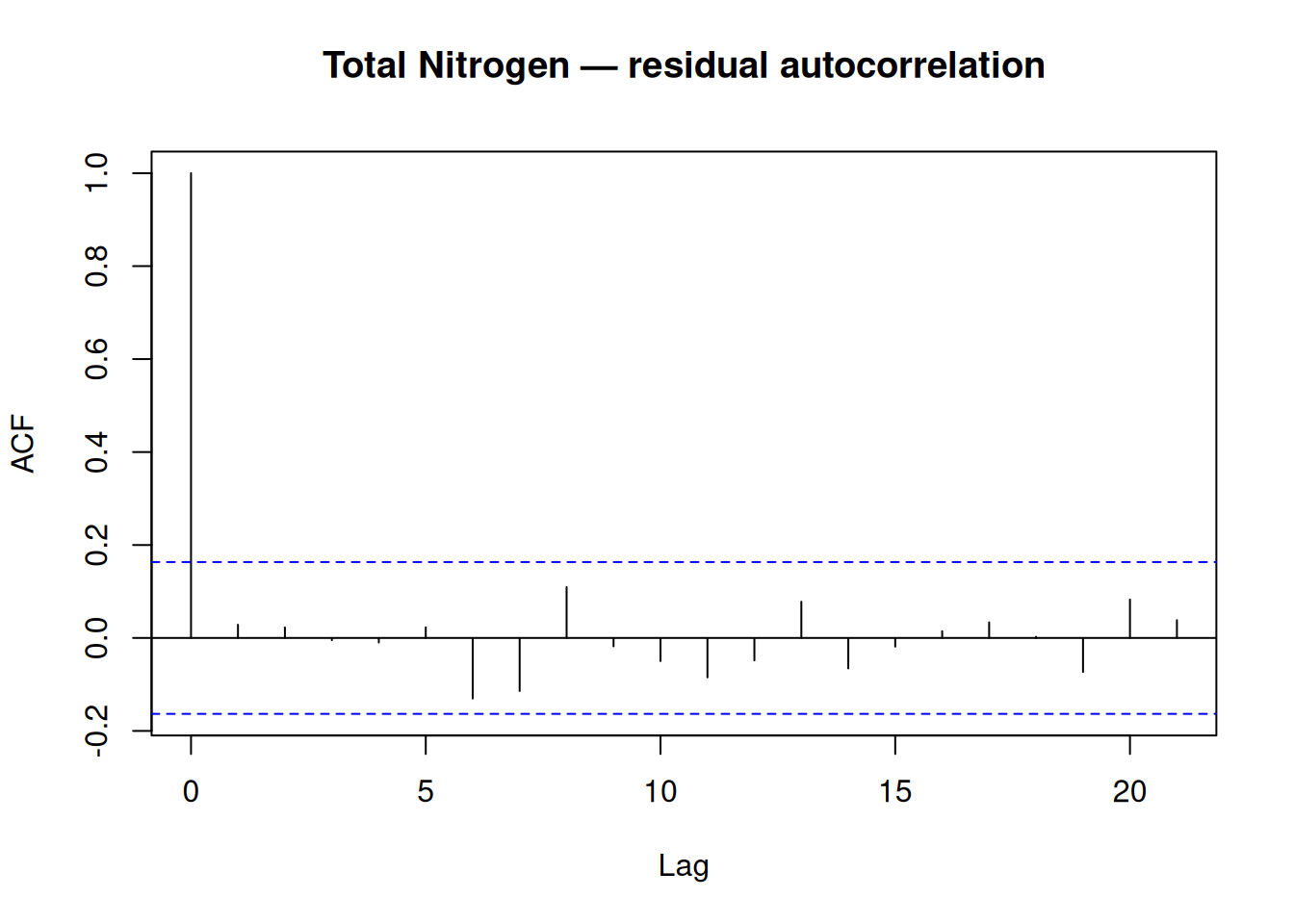
Box.test(resid(seg_tn), lag = 1, type = "Ljung-Box")
    Box-Ljung test

data:  resid(seg_tn)
X-squared = 0.11865, df = 1, p-value = 0.7305
Autocorrelation at lag \(k\) is the correlation between each residual and the residual \(k\) observations earlier, \(\hat e_t\) vs. \(\hat e_{t-k}\); lag-1 is that correlation one month back. A value near zero means this month’s residual carries no information about last month’s — consecutive readings aren’t tracking each other beyond what the fitted trend already explains.
The Ljung-Box test makes that formal: \(H_0\) is that the residuals are independent (no autocorrelation at the lags tested), assessed by pooling the squared autocorrelations across those lags into a single statistic — a low p-value means at least one of them is too large to be noise.
Lag-1 autocorrelation is close to zero, and the Ljung-Box test finds no evidence against independence (\(p = 0.731\)). Nothing here argues for revisiting the segmented fit’s standard errors the way GAMM has to for Dissolved Oxygen.
Total Nitrogen was flat for roughly the first six years of the record and then began rising at approximately 15% per year, with the shift estimated — not assumed — at year_frac ≈ 5.9, about six years into the twelve-year record, with a residual uncertainty band of roughly ±0.7 years around that estimate. The pre-break segment shows no detectable trend; the post-break segment’s rate is estimated precisely enough (95% CI 0.120–0.160 log-units per year) to report with confidence. The model’s assumptions hold up under diagnostic testing, supporting the fit as a defensible basis for the interpretation above.
This fit fully attributes Total Nitrogen’s rise to time alone; a real trend analysis would typically check whether that rise tracks a hydrologic covariate instead — streamflow or precipitation, regressed out before testing for a residual trend — since a wet-weather-driven rise and a genuine loading increase call for different conclusions, and single-covariate time trends like this one can’t distinguish them.