ggplot(cond, aes(year_frac, log(result))) +
  geom_point(alpha = 0.5) +
  geom_smooth(se = FALSE) +
  labs(title = "Specific Conductance — log scale") +
  nlt_theme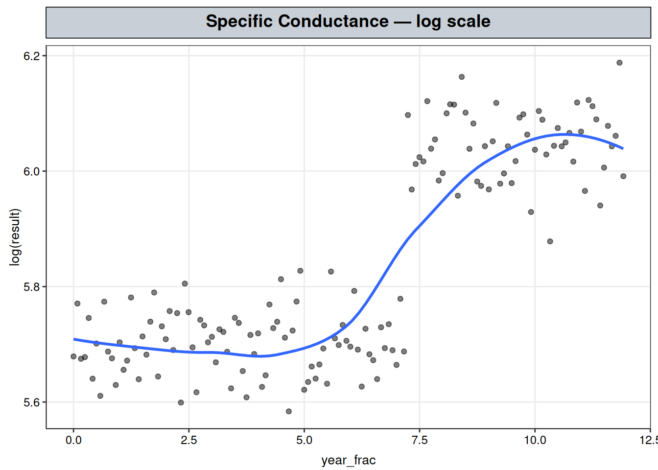
Specific Conductance — a level shift at an unknown point
Piecewise regression (previous chapter) assumes a slope on at least one side of the knot and asks how much it changes. Specific Conductance, explored here, doesn’t fit that setup: it holds at one level, then jumps to another, with no slope (i.e., flat) on either side. Testing for a change in slope like with piecewise regression would find nothing because there isn’t one; what changed is the mean itself.
That’s the piecewise-constant case from Piecewise Regression’s three-stage progression: each segment gets its own flat mean, no slope term on either side. Changepoint detection fits that same piecewise-constant model, but treats the knot’s location as unknown and estimates it from the data, rather than fixing it in advance the way that chapter’s progression assumed.
The strucchange package provides that search. Given a formula and a series, it tests whether a break exists at all, locates it if so, and reports a confidence interval on where — three tools that will be explored through this chapter (Fstats()/sctest(), breakpoints(), and confint()).
In R’s formula notation, the 1 on the right-hand side of y ~ 1 stands for the intercept term alone — no regressor, just \(y_i = \beta_0 + \varepsilon_i\). Fit that model, lm(y ~ 1), on a set of points and it estimates the one coefficient, \(\hat\beta_0\), by minimizing the sum of squared residuals \(\sum (y_i - \hat\beta_0)^2\).
Differentiate with respect to \(\hat\beta_0\), set it to zero, and the minimizer is \(\hat\beta_0 = \bar y\) — the sample mean. An intercept-only regression on a subset of points and the arithmetic mean of that subset are the same number, arrived at by the same minimization, just described two different ways — so each segment’s mean is legitimately an OLS fit rather than an approximation to one. lm(log(result) ~ period) in the Results section below does the same thing with one more coefficient — a shared baseline plus an offset for the second segment — still fit by minimizing squared residuals, which is why it’s still legitimate to call this a regression rather than a two-sample test dressed up as one.
For a single break at position \(\tau\) in the observation sequence, the flat-mean version of this is
\[y_i = \mu_1 \, \mathbb{1}(i \le \tau) + \mu_2 \, \mathbb{1}(i > \tau) + \varepsilon_i,\]
two segment means and an indicator for which segment each observation falls in — exactly the lm(log(result) ~ period) fit in the Results section below, once \(\tau\) is known. The estimation problem is finding \(\hat\tau\) itself:
\[\hat\tau = \arg\min_{\tau} \; \mathrm{RSS}(\tau), \qquad \mathrm{RSS}(\tau) = \sum_{i \le \tau} (y_i - \bar y_{\le \tau})^2 + \sum_{i > \tau} (y_i - \bar y_{> \tau})^2,\]
\(\mathrm{RSS}(\tau)\) is the total squared residual left over once each segment is fit to its own mean — the same quantity OLS always minimizes, just evaluated separately on either side of a candidate split \(\tau\).
\(\hat\tau\) is whichever split leaves the smallest such total, out of every admissible split. strucchange::breakpoints(), used below to locate the break in Specific Conductance’s record, automates that search: it fits the OLS regression at every admissible location (via the dynamic-programming algorithm of Bai and Perron, 2003) and returns whichever minimizes \(\mathrm{RSS}(\tau)\).
This analysis answers the same question a client or regulator would ask about a suspected operational change: did conductance step up, and by how much, and when? What changepoint detection adds over an eyeballed read is a formal test behind each part of that answer — a significance test for whether a break exists at all (sctest() below), a location with a confidence interval, and a percentage change in level with its own p-value.
The situation this method is built for is a suspected step change with an unrecorded date — an operational change, a new discharge starting, a permit-limit revision, a lab or method switch — where there’s reason to think something shifted but no on-record date to seed a local search with. segmented(), from the piecewise regression chapter, needs a plausible starting guess close to the true knot to converge correctly; breakpoints()’s exhaustive search doesn’t need one, which makes it the better first-pass tool for an undocumented shift, or for screening many series at once without eyeballing each one first.
ggplot(cond, aes(year_frac, log(result))) +
geom_point(alpha = 0.5) +
geom_smooth(se = FALSE) +
labs(title = "Specific Conductance — log scale") +
nlt_theme
Flat, then a step up, with no visible slope change on either side of the jump.
Before locating anything, it’s worth testing whether a break exists at all, rather than assuming one and going straight to where it is. The supF test scans every candidate split point and asks whether the best of them fits meaningfully better than a single flat mean across the whole record.
fs <- Fstats(log(result) ~ 1, data = cond)
sctest(fs, type = "supF")
    supF test

data:  fs
sup.F = 1244.3, p-value < 2.2e-16
The test rejects the no-break null decisively (\(p < 2.2 \times 10^{-16}\)): some split in the record explains the data far better than treating it as one constant mean throughout.
Two things need to be uncovered: how many breaks the record has, and whether each segment should be modelled as a flat mean or as its own slope. breakpoints() fits the optimal partition for a given number of breaks; BIC is used twice below to make both choices — once across increasing break counts, and once between the two segment forms.
An intercept-only fit, bp_mean below (breakpoints(log(result) ~ 1)), assumes a flat mean within each segment. If the data actually trended up or down within a segment, that flat line wouldn’t track it.
That assumption belongs to the formula, not to breakpoints() itself — the function accepts any regression formula, so it doesn’t force flat segments over sloped ones or the reverse. Handed ~ year_frac instead, it fits bp_slope (breakpoints(log(result) ~ year_frac)), a non-continuous piecewise-linear model with its own slope and intercept per segment, the knot still found by search.
Trying both and letting BIC pick between them, below, is how the choice gets made without assuming it upfront.
BIC scores a fitted model by its goodness of fit minus a penalty for each added parameter, so it’s the standard way to compare two models with different numbers of parameters without the more flexible one automatically winning just for having more of them; the lower-BIC model is preferred. If slopes actually mattered here, bp_slope’s better fit would outweigh its extra-parameter penalty and win on BIC, and the write-up would report two rates the way Piecewise Regression does, instead of one level jump.
bp_mean <- breakpoints(log(result) ~ 1, data = cond)
bp_slope <- breakpoints(log(result) ~ year_frac, data = cond)

summary(bp_mean)
     Optimal (m+1)-segment partition:

Call:
breakpoints.formula(formula = log(result) ~ 1, data = cond)

Breakpoints at observation number:

m = 1            87
m = 2         60 87
m = 3   21    60 87
m = 4   21    60 87 121
m = 5   21 44 66 87 121

Corresponding to breakdates:

m = 1                                                         0.604166666666667
m = 2                                       0.416666666666667 0.604166666666667
m = 3   0.145833333333333                   0.416666666666667 0.604166666666667
m = 4   0.145833333333333                   0.416666666666667 0.604166666666667
m = 5   0.145833333333333 0.305555555555556 0.458333333333333 0.604166666666667

m = 1
m = 2
m = 3
m = 4   0.840277777777778
m = 5   0.840277777777778

Fit:

m   0         1         2         3         4         5
RSS    4.5424    0.4653    0.4634    0.4596    0.4578    0.4579
BIC -79.1224 -397.2926 -387.9288 -379.1907 -369.8043 -359.8254summary(bp_slope)
     Optimal (m+1)-segment partition:

Call:
breakpoints.formula(formula = log(result) ~ year_frac, data = cond)

Breakpoints at observation number:

m = 1            87
m = 2         60 87
m = 3      39 60 87
m = 4      39 60 87 111
m = 5   21 42 66 87 111

Corresponding to breakdates:

m = 1                                                         0.604166666666667
m = 2                                       0.416666666666667 0.604166666666667
m = 3                     0.270833333333333 0.416666666666667 0.604166666666667
m = 4                     0.270833333333333 0.416666666666667 0.604166666666667
m = 5   0.145833333333333 0.291666666666667 0.458333333333333 0.604166666666667

m = 1
m = 2
m = 3
m = 4   0.770833333333333
m = 5   0.770833333333333

Fit:

m   0         1         2         3         4         5
RSS    1.5755    0.4644    0.4542    0.4450    0.4385    0.4495
BIC -226.6288 -387.6206 -375.9216 -363.9415 -351.1634 -332.6749
bp_mean and bp_slope select the same single breakpoint at observation 87, and both agree it’s the best choice of break count. They disagree on whether that break should carry a slope: at one break, bp_mean’s BIC (-397.3) is lower than bp_slope’s (-387.6). Adding two slope parameters costs more in complexity than it recovers in fit, confirming the data-driven version of what the raw plot already suggested: a level shift, distinct from a change in trend.
Therefore, based on the evaluation of the model results, bp_mean is carried forward.
ci <- confint(bp_mean)
ci
     Confidence intervals for breakpoints
     of optimal 2-segment partition:

Call:
confint.breakpointsfull(object = bp_mean)

Breakpoints at observation number:
  2.5 % breakpoints 97.5 %
1    86          87     88

Corresponding to breakdates:
      2.5 % breakpoints    97.5 %
1 0.5972222   0.6041667 0.6111111
brk_idx <- ci$confint[, "breakpoints"]
cond$year_frac[ci$confint[, c("2.5 %", "breakpoints", "97.5 %")]][1] 7.082820 7.162218 7.247091The breakpoint falls at observation 87, year_frac ≈ 7.16 (95% CI 7.08–7.25) — a little over seven years into the twelve-year record. strucchange’s convention is that the reported observation is the last one belonging to the first segment, so the split is applied as strictly-after that index below.
bp_mean already fits a mean per segment, but its coefficients are on the log scale and don’t come with a ready percent-change figure. Refitting the same intercept-only split as an explicit two-level factor makes that conversion straightforward: exponentiate each segment’s mean, then take the percent difference between them.
# strictly after brk_idx, matching strucchange's "last obs of first segment" convention
period <- factor(seq_along(cond$year_frac) > brk_idx, labels = c("before", "after"))
fit <- lm(log(result) ~ period, data = cond)
summary(fit)
Call:
lm(formula = log(result) ~ period, data = cond)

Residuals:
      Min        1Q    Median        3Q       Max
-0.166308 -0.038616 -0.001541  0.038538  0.143264

Coefficients:
            Estimate Std. Error t value Pr(>|t|)
(Intercept) 5.700487   0.006137  928.87   <2e-16 ***
periodafter 0.344080   0.009754   35.27   <2e-16 ***
---
Signif. codes:  0 '***' 0.001 '**' 0.01 '*' 0.05 '.' 0.1 ' ' 1

Residual standard error: 0.05724 on 142 degrees of freedom
Multiple R-squared:  0.8976,    Adjusted R-squared:  0.8968
F-statistic:  1244 on 1 and 142 DF,  p-value: < 2.2e-16
R codes period against its first level, before, so (Intercept) is the mean of log(result) in the before segment (5.70), and periodafter is the difference the after segment adds to it (0.344). Both are on the log scale and in units of log(result), which is why they don’t read as a plain before/after comparison yet.
The intercept’s p-value isn’t of interest: it tests whether the before-segment mean is zero, a null with no substantive meaning here (log(result) = 0 would mean the raw analyte equals 1, an arbitrary reference point, not “no effect”). periodafter’s p-value is the one that matters — it tests whether the after segment differs from the before segment at all, which is the claim this section is making, and it’s highly significant (\(p < 2\times10^{-16}\)).
fit established that the two segments differ —and by how much —on the log scale, but a client or regulator wants the answer in the analyte’s own units: a level and a percent change, not a log-scale coefficient. Getting there takes two steps: recover each segment’s mean in raw units, then convert the difference between them to a percentage.
# same two numbers as fit's coefficients (5.70, 5.70 + 0.344), computed directly as group means
means <- tapply(log(cond$result), period, mean)
exp(means) # undoes the log — segment means back in the analyte's raw units
before after
299.0130 421.8149 pct_jump <- (exp(diff(means)) - 1) * 100 # exp() of the log-scale difference gives a ratio; -1 converts it to a percent
pct_jump after
41.0691 means holds the same two numbers fit already estimated — 5.70 for before, 6.04 (5.70 + 0.344) for after — computed here as plain group averages of log(result) rather than read off the model’s coefficients, so there’s no need to track which coefficient is the intercept and which is the offset.
exp(means) returns the two segment means in the analyte’s raw units: about 299 before, about 422 after. These are geometric means — the back-transform of an average taken on the log scale — not arithmetic means of the raw values, which is the correct summary here since bp_mean and fit were both fit on log(result).
exp(diff(means)) instead exponentiates the 0.344 log-scale difference between the two means, converting it to a ratio between segments rather than to either mean individually; subtracting 1 turns that ratio into a percent change — roughly a 41% jump.
cond_pred <- cond |> mutate(fitted = predict(fit))
brk_year <- cond$year_frac[brk_idx]
ci_years <- cond$year_frac[ci$confint[, c("2.5 %", "97.5 %")]]

ggplot(cond, aes(year_frac, log(result))) +
  annotate("rect", xmin = ci_years[1], xmax = ci_years[2], ymin = -Inf, ymax = Inf,
           fill = "grey70", alpha = 0.4) +
  geom_point(alpha = 0.5) +
  geom_line(data = cond_pred, aes(y = fitted, group = period), color = "steelblue", linewidth = 1) +
  geom_vline(xintercept = brk_year, linetype = "dashed") +
  annotate(
    "label",
    x = brk_year + 0.2, y = max(log(cond$result)),
    label = sprintf("Break = %.2f yr, Jump = %.1f%%", brk_year, pct_jump),
    hjust = 0, vjust = 1, size = 3.6
  ) +
  labs(title = "Specific Conductance — mean-shift fit (log scale)") +
  nlt_theme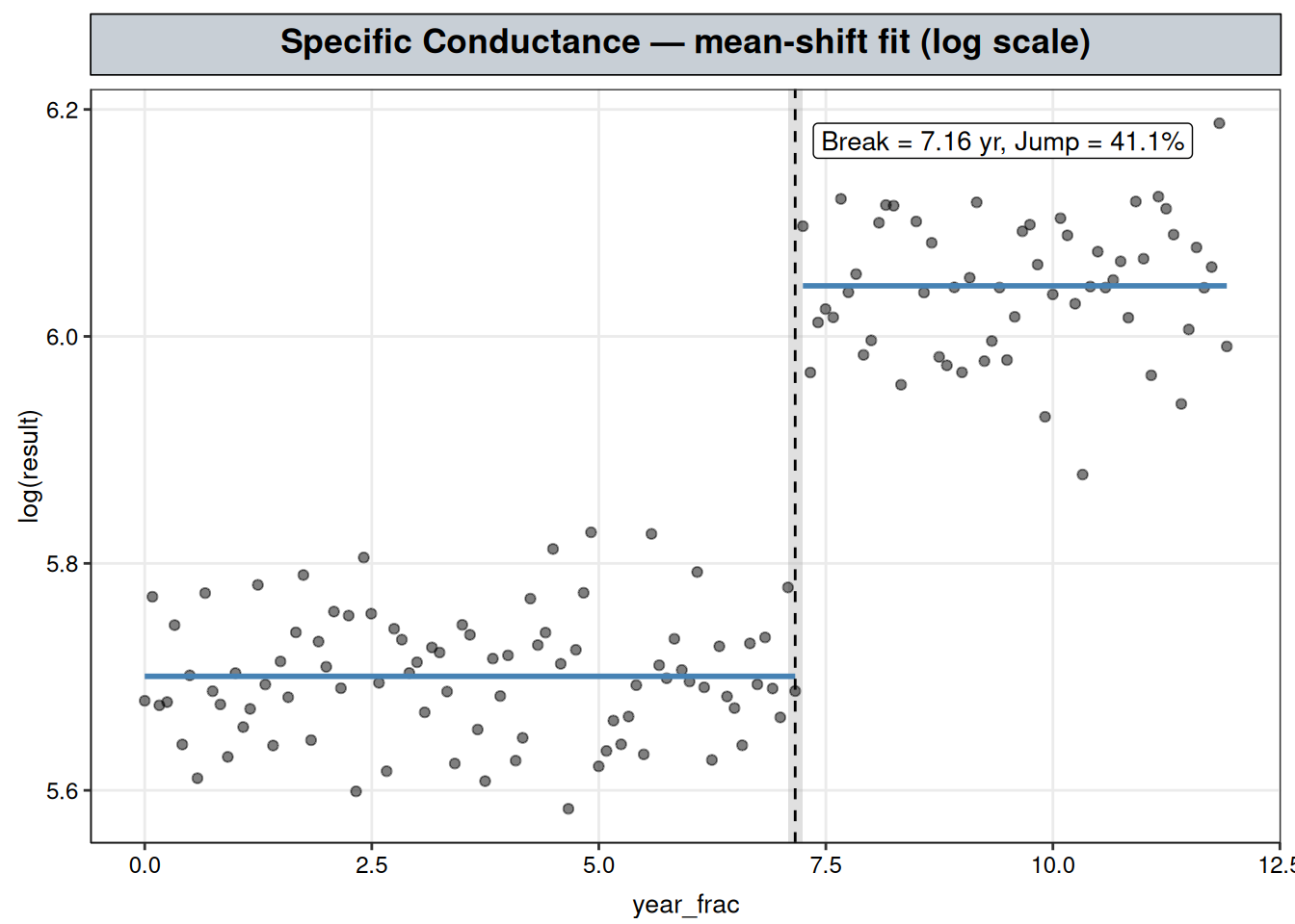
The two-segment fit is still an OLS regression, so the same assumptions apply: homoscedasticity and normally distributed residuals (see Transformations).
bptest(fit)
    studentized Breusch-Pagan test

data:  fit
BP = 1.1391, df = 1, p-value = 0.2858shapiro.test(resid(fit))
    Shapiro-Wilk normality test

data:  resid(fit)
W = 0.99481, p-value = 0.8889
Both tests fail to reject their null: the Breusch-Pagan test (\(p = 0.286\)) finds no evidence of heteroscedasticity, and the Shapiro-Wilk test (\(p = 0.889\)) finds no evidence of non-normal residuals.
acf(resid(fit), main = "Specific Conductance — residual autocorrelation")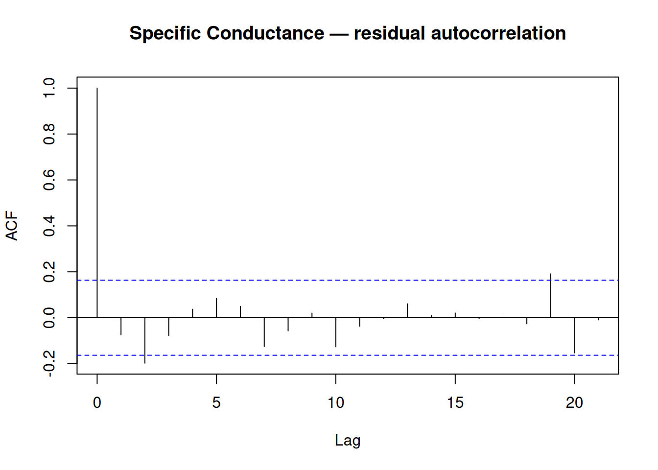
Box.test(resid(fit), lag = 1, type = "Ljung-Box")
    Box-Ljung test

data:  resid(fit)
X-squared = 0.80978, df = 1, p-value = 0.3682
Lag-1 autocorrelation is close to zero and the Ljung-Box test finds no evidence against independence (\(p = 0.368\)).
All three assumptions hold, supporting the fit as a defensible basis for the interpretation below.
Specific Conductance held at a stable level for the first seven-plus years of the record, then stepped up to a new, equally stable level, with the shift located at year_frac ≈ 7.16 (95% CI 7.08–7.25).
Unlike the piecewise-regression case, no slope was fit or needed on either side of the break: comparing a flat-mean model against a slope-and-intercept model at the same breakpoint showed that the added slope terms cost more in model complexity than they gained in fit, confirming this is a level shift rather than a change in trend. The jump itself is large and precisely estimated — the mean level rises by roughly 41%, from about 299 to about 422 — and the diagnostics support treating the two-segment fit as a defensible basis for that reading.
Locating the break statistically is only half of what a regulator or client actually wants — the next step is attribution: checking the estimated date (year_frac ≈ 7.16, roughly year 2020) against operational logs, permit modifications, or upstream discharge records to see what happened around then. Nothing in this analysis can supply that on its own; the break’s confidence interval narrows where to look, not why it happened. If several analytes or several monitoring sites are believed to share a common cause, it’s also worth testing whether the same breakpoint shows up in more than one series at once — breakpoints() fits each series independently here, but a shared-cause hypothesis is really a claim about a common changepoint across series, which calls for a joint test rather than eyeballing whether several independently-estimated dates happen to be close.