Diagnosing why a response resists a straight line, and matching the correction to the actual cause
Before reaching for one of the heavier models later on this site — piecewise regression, changepoint detection, GAMs — a series deserves a simpler question: is it really nonlinear, or is it a straight line on the wrong scale? A simpler model that fits is generally the better model — fewer parameters to estimate, easier to explain, more likely to generalize beyond the data it was fit on. This chapter is that correction step.
By correction I mean a targeted change to how the straight-line model is set up — one that lets an ordinary linear fit describe a shape it couldn’t handle as given, without switching to a different method.
Three such corrections exist: transform the response, feature-engineer the regressor, or change the link function. What follows is how to read a series’s raw shape and residuals to tell which one applies, if any, using the five-part model from The Regression Framework to pin down where each acts.
1 Matching the correction to the cause
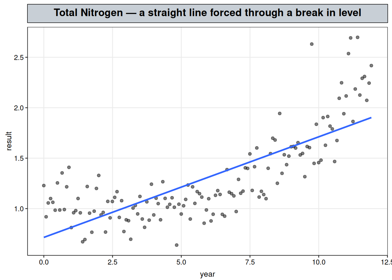
A response with a restricted range — a concentration, which can’t go negative — routinely needs some kind of correction before ordinary least squares is a defensible fit. Total Nitrogen is a case in point: flat for the first several years of the record, then rising. A straight line fit to it anyway captures neither stretch well.
tn_raw <- non_linear_wq |>filter(analyte =="Total Nitrogen")ggplot(tn_raw, aes(year_frac, result)) +geom_point(alpha =0.5) +geom_smooth(method ="lm", se =FALSE) +labs(title ="Total Nitrogen — a straight line forced through a break in level",x ="year", y ="result") + nlt_theme
`geom_smooth()` using formula = 'y ~ x'
The line is a compromise between two regimes it was never built to describe — too high early, too low late, too shallow in between. Which correction fixes that depends on where the problem actually sits.
Three techniques address these separately, and they are easy to conflate because more than one can involve the word “log” — but they are not interchangeable, and reaching for the wrong one leaves the real problem uncorrected.
Instead of a typical OLS model of lm(result ~ year_frac), corrections could be made by:
Transform the response — log(result) instead of result. This changes OLS’s estimand: the fitted mean becomes the conditional mean of log(result) instead of result. It’s a data preparation step, done before the model ever sees the numbers.
Feature-engineer the regressor — for example, a hinge term pmax(0, year_frac - c) for a series whose slope itself changes partway through the record. This changes the shape of the systematic component while leaving the response and the link alone. Still OLS, still linear in the coefficients (see The Regression Framework) — just an additional regressor handed to lm().
Change the link function — a generalized linear model with a log link function, \(\log(E[Y\mid X]) = X\beta\). This changes how the mean relates to the linear predictor rather than the response itself.
The first and third both involve the word “log” applied to a concentration, but they aren’t the same model: \(E[\log(Y)\mid X]\) (log-transform-then-OLS) and \(\log(E[Y\mid X])\) (a GLM log link) are different quantities and only coincide in special cases.
Concentration data is generated by processes — dilution, loading, removal — that act as a percentage change on the current level rather than a fixed absolute amount (the multiplicative-process argument developed in full below), and that structure is what log-transform-then-OLS is built to estimate: it puts the model directly on the scale where a percentage-change process produces additive, symmetric noise.
A log-link GLM instead assumes the mean itself is multiplicative in the predictors while the noise stays additive on the raw scale — a different, also defensible assumption. However, the USEPA recommends the standard of log-transform-then-OLS rather than a log-link GLM for temporal trends (proUCL); so, even though a log-link GLM remains a reasonable alternative, it is less commonly used by environmental scientists.
The rest of this chapter works through these in order: how to tell, from the raw data and from residual diagnostics, whether a series needs the response transformed or the regressor feature-engineered; why log-transform-then-OLS in particular fits the multiplicative-process story environmental concentration data tends to follow; and, at the end, the narrower case where the log-link GLM is worth revisiting after all — paired with Gamma rather than Gaussian noise, when the deliverable is a raw-scale mean rather than a %/year rate.
2 Deciding between response-transform and the regressor-feature-engineering corrections
The response-transform and the regressor-feature-engineering questions get resolved separately, in a fixed order, because they fail differently.
2.1 Step 1 — look at the raw shape before touching residuals
log() is a monotonic transform, so it can only re-scale curvature that’s already headed one direction — it can straighten an accelerating or decaying curve, but it cannot introduce a bend, a peak, or a flattening that isn’t there on the raw scale, and it cannot remove one that is. That splits raw-shape curvature into two cases:
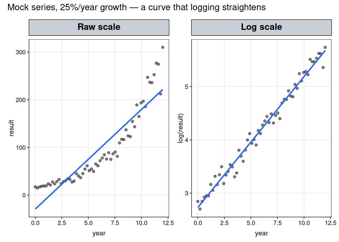
Monotonic curvature that logging fixes: a quantity growing (or decaying) at a fixed percentage rate per period — i.e. exponential growth/decay, \(y = Ae^{rt}\) — is curved on the raw scale but linear once logged: \(\log(y) = \log(A) + rt\). The panels below are a mock series at a 25%/year rate — unrealistically steep for real environmental chemistry, chosen purely to make the curvature-then-straightening visible.
Non-monotonic shapes — a plateau, a kink, a hump, or any curve that doesn’t move consistently in one direction. These signal a need to feature-engineer the regressor instead of reaching for log(); no response transform fixes them.
On the raw scale the fitted line overshoots the middle of the record and undershoots both ends — a signature of forcing a straight line through what’s actually an accelerating curve. On the log scale the same line runs through the data cleanly: this is the case Step 1 is checking log(result) for.
2.2 Step 2 — fit the straight line anyway, and read the residuals, not the raw data
The residual for observation \(i\) is the gap between what was observed and what the fitted line predicts, \(\hat{e}_i = y_i - \hat{y}_i\) — the vertical distance from a point to the fitted line, plotted directly in the systematic-vs-random-component figure in The Regression Framework. A correctly specified model leaves residuals that look like patternless, constant-variance noise; how they depart from that is what tells you which correction is needed.
Two different things can go wrong once the residuals are examined, and they matter for different reasons — one means the fitted line itself is in the wrong place, the other means the line might be fine but the uncertainty claimed around it isn’t:
A regressor problem. Residuals show a pattern against the regressor: systematically high in some stretches and low in others, rather than scattered evenly. That means the fitted mean is the wrong shape: the line doesn’t track the data’s true curve, so the slope or rate read off it is biased rather than merely imprecise. This is the more serious failure, because it means the headline number is wrong.
A distributional problem. Residuals look patternless against the regressor — the mean structure is fine — but their spread grows with the fitted value, or their distribution departs from normal. Here the fitted mean can be trusted, but the confidence intervals and p-values built on top of it assume constant-variance, normally distributed noise, and stop being trustworthy once that assumption breaks. The point estimate can still be trusted; the confidence interval around it cannot.
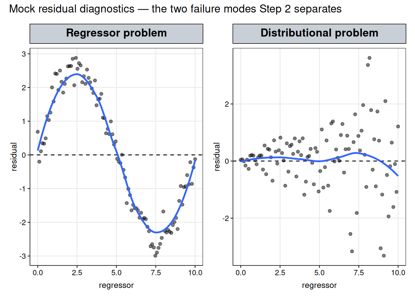
The left panel is a mock: a smooth systematic wave, the smoother tracking well away from zero across stretches of the regressor — the signature of a mean structure that hasn’t captured the true shape yet, no amount of response-transforming fixes this.
The right panel is also a mock: the smoother stays flat on zero (no shape has been missed), but the scatter visibly widens as the regressor increases — a distributional problem the response side of the model is meant to handle.
Breusch-Pagan and Shapiro-Wilk are formal tests for the distributional problem only — neither one checks whether the mean structure is right, so neither one can catch a regressor problem:
Breusch-Pagan tests \(H_0\): the residual variance is constant across fitted values (homoscedasticity), by regressing the squared residuals on the fitted values and testing whether that regression has any real explanatory power. A low p-value means the spread is changing — the residuals are fanning in or out.
Shapiro-Wilk tests \(H_0\): the residuals are drawn from a normal distribution, by comparing the sample’s order statistics against the quantiles a normal distribution would produce. A low p-value means the residual distribution’s shape — skew, heavy tails, multimodality — departs from normal.
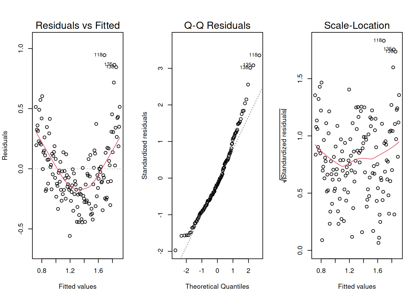
A regressor problem has no formal test at all — it has to be seen. Base R’s plot() on a fitted model produces this directly, alongside the two panels that back up Breusch-Pagan and Shapiro-Wilk:
fit_tn_naive <-lm(result ~ year_frac, data = tn_raw)par(mfrow =c(1, 3))plot(fit_tn_naive, which =1)plot(fit_tn_naive, which =2)plot(fit_tn_naive, which =3)
Residuals vs Fitted (which = 1) is the regressor-problem check — with a single regressor, fitted values are a monotonic function of it, so a pattern here is the same pattern a plot against the raw regressor would show; this is the one panel neither formal test looks at. Normal Q-Q (which = 2) is the visual companion to Shapiro-Wilk: points following the diagonal mean the residual distribution is close to normal, systematic curvature or S-shapes mean it isn’t. Scale-Location (which = 3) is the visual companion to Breusch-Pagan: a flat trend means constant variance, an upward slope means it’s fanning out.
2.3 The bridge to a fully flexible regressor
A hinge function, \((x-c)_+ = \max(0, x-c)\), is the simplest possible case of feature-engineering the regressor: one knot, one new column, still fit by lm(). A generalized additive model’s smooth term generalizes the same idea — many small basis functions instead of one hinge, combined additively, with a fitted penalty deciding how much of that flexibility survives rather than an analyst placing knots by eye. The lineage is straight-line OLS \(\to\) hinge-term feature engineering \(\to\) many-basis-function smooth term, and it’s the same “linear in the parameters” backbone the whole way — what changes across that lineage is how many, and how flexible, the basis functions handed to the fit are allowed to be.
3 Log-transform-then-OLS for concentration data
3.1 Why log a concentration in the first place
The multiplicative argument for environmental chemistry is that concentration data is strictly positive, and the processes that move it — dilution, loading, removal — tend to act as a fixed percentage change on the current level rather than a fixed absolute amount. A process like that generates a distribution that’s approximately log-normal by construction: right-skewed on the raw scale, closer to symmetric once logged. Fitting log(result) rather than result is what typically fixes the two ordinary-least-squares assumptions raw concentration data tends to violate — homoscedasticity and normality of residuals
A coefficient estimated on log(result) is a rate in log-units per period, and back-transforming it, \((\exp(\hat\beta) - 1) \times 100\%\), gives the number that actually gets reported — a constant percentage rate of change, not a raw-unit slope.
3.2 When a Gamma GLM is the better call
Recall the log-link GLM from the third correction option at the top of this chapter, \(\log(E[Y\mid X]) = X\beta\): it was paired there with ordinary (Gaussian) noise, then set aside in favor of log-transform-then-OLS as the USEPA/proUCL standard.
This section asks a narrower question: what if the log link is kept, but the noise assumption is swapped for one that actually matches concentration data’s multiplicative behavior? The result is a Gamma GLM — a fitted mean on the raw concentration scale directly, with no back-transformation step and no bias to correct for.
The earlier default doesn’t change for any case study on this site — log-transform-then-OLS stays the standard fit throughout, and reporting a %/year rate off the log scale never runs into the problem below, since that rate is computed and reported entirely in log units.
The problem: naively exponentiating a log-OLS fit, exp(predict(fit)), is a biased estimate of \(E[Y\mid X]\) — it systematically understates the raw-scale mean. The reason is what’s called Jensen’s gap: log-OLS fits \(E[\log(Y)\mid X]\), but exponentiating that gives \(\exp(E[\log(Y)\mid X])\), not \(E[Y\mid X]\) — and because \(\exp()\) is a convex function, those two are different quantities in general (this is the same \(E[\log(Y)\mid X])\) vs. \(\log(E[Y\mid X])\) distinction raised earlier in this chapter).
A Gamma GLM sidesteps the problem rather than correcting for it: because it’s fit directly to \(E[Y\mid X]\) rather than reached by exponentiating a fit to \(E[\log(Y)\mid X]\), its raw-scale mean is unbiased with nothing to fix afterward. That’s the specific case where a Gamma GLM earns its place over log-transform-then-OLS: whenever the deliverable is that raw-scale mean itself, rather than a log-scale rate.
A GLM is specified by two separate pieces, and it’s the pairing of the two that determines whether the noise ends up additive or multiplicative:
Link function — how the mean relates to the linear predictor. A log link, \(\log(E[Y\mid X]) = X\beta\), makes the mean multiplicative in the predictors: \(E[Y\mid X] = \exp(X\beta)\). This is a statement about the mean only; it says nothing about how the noise around that mean behaves.
Family / variance function — how the variance relates to the mean, \(\mathrm{Var}(Y\mid X) = \phi\, V(\mu)\). Here \(\phi\) is the dispersion parameter — a single constant, estimated from the data, that scales the variance up or down without changing its shape — and \(V(\mu)\) is the family-specific function of the mean that this table sets out. Family/variance-function is a separate choice from the link, and it’s what actually determines whether the noise is additive or multiplicative.
Table 1: How the family choice sets the mean-variance relationship, holding the log link fixed
Family
Variance function \(V(\mu)\)
Noise behavior
Gaussian
\(V(\mu) = 1\) (constant)
Additive — spread stays the same size regardless of the mean level
Gamma
\(V(\mu) = \mu^2\)
Multiplicative — spread scales with the square of the mean
The log-link GLM introduced above pairs a log link with a Gaussian family — multiplicative mean, but Gaussian’s constant-variance noise stays additive, not the structure a percentage-change process actually produces. Swapping the family to Gamma while keeping the log link changes nothing about the mean structure (\(E[Y\mid X] = \exp(X\beta)\) either way) but changes the noise from additive to multiplicative: \(\mathrm{Var}(Y\mid X) = \phi\, E[Y\mid X]^2\), variance growing with the square of the mean rather than staying fixed. That pairing — log link for the mean, Gamma family for the noise — is a much closer match to concentration data’s actual behavior, and it comes with a real advantage log-transform-then-OLS doesn’t have: the Gamma GLM’s fitted mean is \(E[Y\mid X]\) directly, on the raw concentration scale, with no back-transformation step at all.
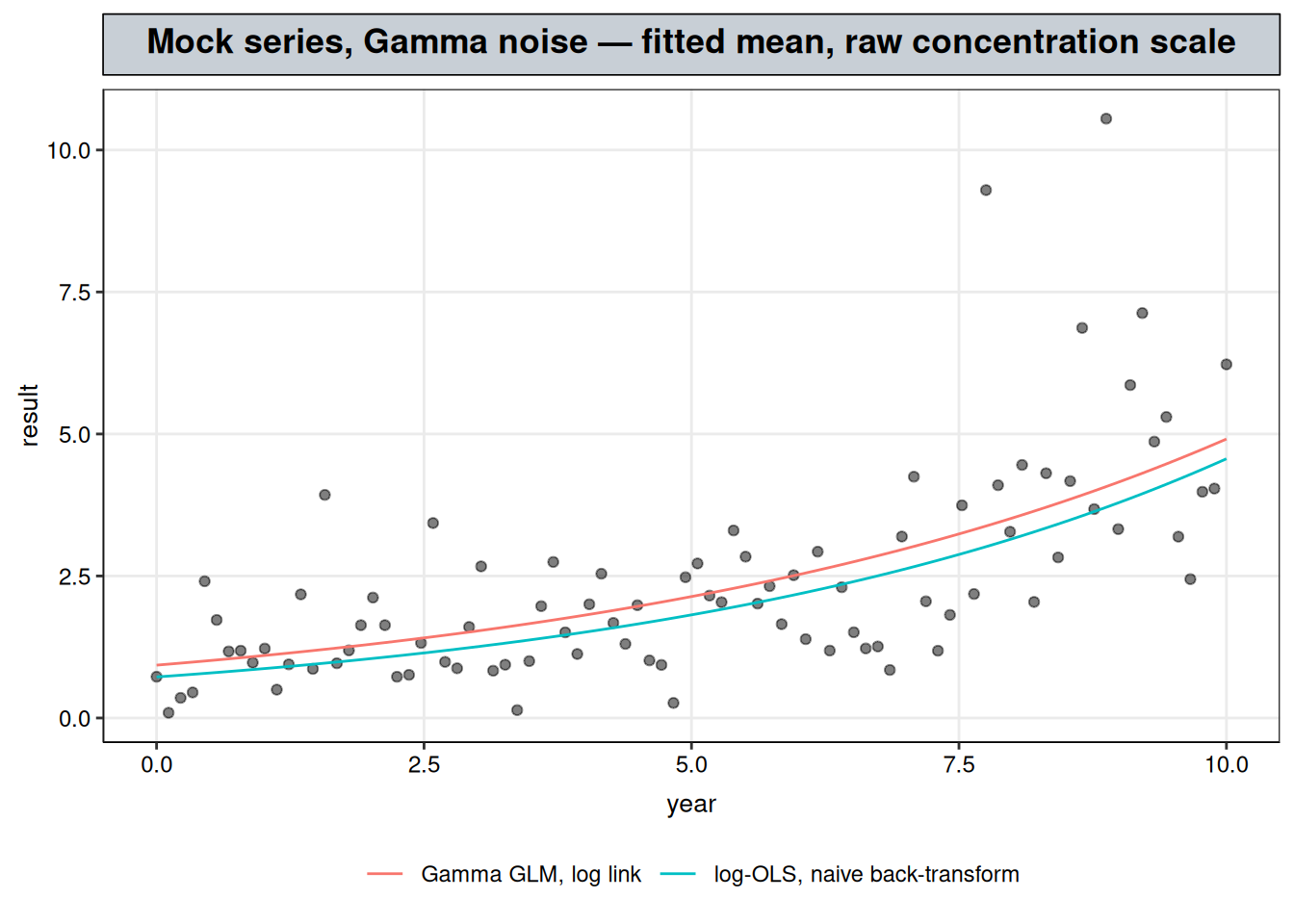
That advantage is the Jensen’s-gap problem described above, made precise: for Gamma-distributed noise specifically, the naive back-transform’s bias is a fixed, calculable amount (\(\psi(\text{shape}) - \log(\text{shape})\), always negative). A mock series makes the gap concrete: a synthetic rising trend, built for this purpose rather than drawn from this site’s case-study analytes, with Gamma noise constructed to have \(\mathrm{Var}(Y) = \phi\mu^2\):
ggplot(mock_gamma, aes(year_frac, result)) +geom_point(alpha =0.5) +geom_line(aes(y = fit_naive, color ="log-OLS, naive back-transform")) +geom_line(aes(y = fit_glm, color ="Gamma GLM, log link")) +labs(title ="Mock series, Gamma noise — fitted mean, raw concentration scale",x ="year", y ="result", color =NULL) + nlt_theme +theme(legend.position ="bottom")
The naive back-transformed log-OLS curve sits visibly below both the Gamma GLM curve and the data cloud: the estimate is biased, a more serious problem than added noise. The Gamma GLM’s fitted curve is unbiased for \(E[Y\mid X]\) because it is fit to that quantity directly, rather than reached by exponentiating a fit to \(E[\log(Y)\mid X]\).
None of this overturns the choice made earlier in this chapter — Total Nitrogen and Total Copper’s residuals are well-behaved enough on the log scale (Breusch-Pagan and Shapiro-Wilk both pass, or fail for shape reasons unrelated to the response transform) that log-transform-then-OLS is a defensible, simpler fit, and every case study on this site stays with it for consistency. Reach for a Gamma GLM instead when the fitted mean itself needs to be reported on the raw concentration scale without back-transformation bias — for instance, comparing a fitted trend directly against a regulatory concentration threshold — or when the bucketed sample variance tracks \(\phi\mu^2\) more closely than the lognormal-residual assumption does.
3.3 Where this differs from ProUCL’s UCL and BTV statistics
EPA’s ProUCL software also weighs a Gamma distribution against a lognormal one — but for a different problem than the one this chapter addresses. ProUCL’s Gamma-vs-lognormal debate belongs to its Upper Confidence Limit (UCL), Upper Tolerance Limit, and background threshold value (BTV) modules: computing a single population parameter from a time-collapsed sample, often with nondetects handled through Kaplan-Meier estimation. That’s a fixed-in-time point estimate, not a conditional mean modeled as a function of a regressor — a different estimand than any method on this site targets (see The Regression Framework).
ProUCL’s actual counterpart to this chapter is its separate Trend Analysis module, which fits plain OLS on the raw, untransformed response as a function of time and falls back to the nonparametric Mann-Kendall and Theil-Sen tests when normal-residual assumptions fail. That module says nothing about Gamma distributions or response transforms — it targets the same conditional-mean estimand this site does, paired with the same parametric/nonparametric cross-check used in the companion vignette-temporal-trends project (log-transform-then-OLS alongside Mann-Kendall and Sen’s slope, run side by side rather than one replacing the other).
ProUCL’s caution against response transformations is specifically about retransformation bias: back-transforming a log-scale statistic to an absolute raw-scale number used directly in a decision, such as comparing an EPC against a cleanup standard. That’s real and well documented — Land’s H-statistic for a lognormal UCL is known to become unstable once the standard deviation of the log-transformed data exceeds about 1 — and it’s the same Jensen’s-gap issue the Gamma GLM example above demonstrates. This chapter’s log-transform-then-OLS avoids that problem: every fitted rate on this site is reported as a %/year figure, computed and interpreted on the log scale (\((\exp(\hat\beta)-1)\times100\%\)), never back-transformed into an absolute concentration for a decision. Log-transform-then-OLS remains the right tool for that estimand. A Gamma GLM, or ProUCL’s own Gamma-based decision statistics, would only become the more defensible choice if the deliverable here were a raw-scale mean or a formal decision statistic — outside this site’s stated scope of inference on the observed record, not forecasting or regulatory comparison.
4 Summary
This chapter set up how to tell, before fitting anything more elaborate, whether a nonlinear-looking series is fixable with a correction to an ordinary straight-line fit rather than a genuinely different model: raw shape (Step 1) for whether the response needs log(), residual diagnostics (Step 2) for whether the regressor needs feature-engineering instead. For concentration data specifically, log-transform-then-OLS is the default — it matches the multiplicative-process story dilution, loading, and removal actually produce, and it’s the USEPA/proUCL standard. Back-transforming a log-scale fit does carry a bias (Jensen’s gap), and a Gamma GLM is available as a way to avoid it when the deliverable is a raw-scale mean — but that bias is inconsequential to every case study on this site, since results here are reported as %/year rates computed on the log scale, never back-transformed into an absolute concentration. No case study needs the Gamma GLM; it’s covered as the answer to a question a reader doing this kind of analysis will eventually ask, rather than as a step this site’s own trend fits require.
With that diagnostic toolkit in place, the rest of this site stops asking whether a correction to a straight line is enough and starts fitting the methods built for series where it isn’t — piecewise regression, changepoint detection, k-NN, LOESS, GAM, and GAMM, each demonstrated on a case study whose shape a response transform or a hand-engineered regressor can’t capture.