Choosing what to report about a nonlinear trend: how the research question, process, and scope dictate the model
1 A fit is not an explanation
Total Phosphorus was last seen in k-Nearest Neighbors and LOESS, which left it as a rise into a plateau, described without assuming any form for the curve. With the full set of methods now in hand, this chapter returns to that record.
The natural next step is to name that shape: find a curve family that looks like it, fit it, and report its parameters as the result. A rise that levels off resembles a logistic growth curve, and a logistic curve fits this record well.
That step needs more than a good fit. Each parameter of a fitted curve makes a claim about the process behind the record. For a logistic growth curve, that means a ceiling the concentration is approaching, a date the change began, and a rate at which it grew.
Tip
Key point: a curve can match the data closely while the process its parameters describe never took place. A fit is not an explanation.
2 Three inputs to the choice
Each chapter so far has matched a model to a shape seen in the data: a bend, a jump, a plateau. Shape is a useful guide, but it should not decide the model on its own. Three inputs come first:
The question. What number does the decision need: a rate of change, whether the record is still rising, the date a goal will be met? This is the estimand from The Regression Framework.
How the data arose. The physical, chemical and hydrological processes behind the values, and the sampling and laboratory practices that recorded them. Statisticians call this the data-generating process.
How far the answer has to reach. Whether the model only needs to describe the monitored period, or has to say something about years not yet observed (forecasting).
None of these is new to water-quality trend analysis. Hirsch et al. (1991) set out trend analysis as a series of choices that begin with what kind of trend is being tested, such as a step change or a gradual monotonic one. In environmental modelling more broadly, Kelly et al. (2013) list the purpose of a model among the factors that decide which modelling approach fits.
When the question and the process are both well understood, they narrow the choice and give the parameters a physical reading that can be checked. When the process is not well understood, the safer choice is a model that describes the record without claiming to know what produced it.
Crossing the third input (how far the answer has to reach) with how well the process is known gives four situations that help decide on an approach:
Process unknown: describe the shape
Process known and checkable: model the process
Within the record (what happened)
When the record changed, how fast, and whether it is still changing. Model: GAM. Example:Total Phosphorus
The effect of a documented event, such as a change in slope at a known date. Model:Piecewise Regression with the break fixed at that date
Beyond the record (forecasting)
The over-modelling trap: a curve chosen because it fits the data, but its forecast will be dictated by the formula’s assumption, and that may not match the process. Don’t forecast with misleading model. Example:Total Phosphorus as a logistic curve
Fit the model the process implies, check it against held-out data, and project with stated limits. Model: first-order decay. Example:plume
A known process can also be checked, because it makes claims the record could fail. First-order decay after source removal says the log-scale record should be a straight line, and that a rate fitted to the early years should predict the later ones; the plume is tested on both. A curve chosen because it looks like the plot has no such test. It was picked for fitting the shape, so fitting the shape is no evidence for it.
3 Total Phosphorus: three fits, one record
The Total Phosphorus record rises through the middle years and then levels off. The question is the one a regulator would ask of any monitoring record: is it still rising?
Nothing about the site establishes the process. Phosphorus at a sampling point reflects loading from the surrounding land, flow and dilution, release from bed sediments, uptake by plants and algae, and sampling and laboratory variation, all acting at once. The monitoring design does not separate them.
Three models are reasonable to reach for given the shape. The first two each come with a story about what happened; the third does not:
Logistic growth curve. An S-shaped rise from a floor to a ceiling, with four parameters: the floor, the ceiling, the midpoint of the rise, and how quickly it happens. Its story is a gradual approach to a fixed upper limit.
Piecewise linear regression with two breakpoints. The model from Piecewise Regression, with a second breakpoint so the record can level off again. Its story is a change that began on one date and was complete by another, such as a new discharge phased in over a few years.
GAM. The smooth from Generalized Additive Models (Wood, 2017), with its shape estimated from the data and its flexibility set by a fitted penalty. It describes the record without proposing a mechanism.
All three are fit to log(result) with Gaussian errors, so their AICs are comparable. As in Piecewise Regression, segmented() needs a starting guess for each breakpoint (psi), read off the plot: about year 3, where the rise begins, and year 8, where it levels off. The search then estimates the breakpoints from the data, so the guesses only need to be close.
fit_logistic <-nls(log(result) ~SSfpl(year_frac, floor, ceiling, mid, scal), data = tp_wq)fit_piecewise <-segmented(lm(log(result) ~ year_frac, data = tp_wq), seg.Z =~year_frac, psi =c(3, 8))fit_tp_gam <-gam(log(result) ~s(year_frac, bs ="tp", k =20), data = tp_wq, method ="REML")c(AIC_logistic =AIC(fit_logistic), AIC_piecewise =AIC(fit_piecewise), AIC_gam =AIC(fit_tp_gam))
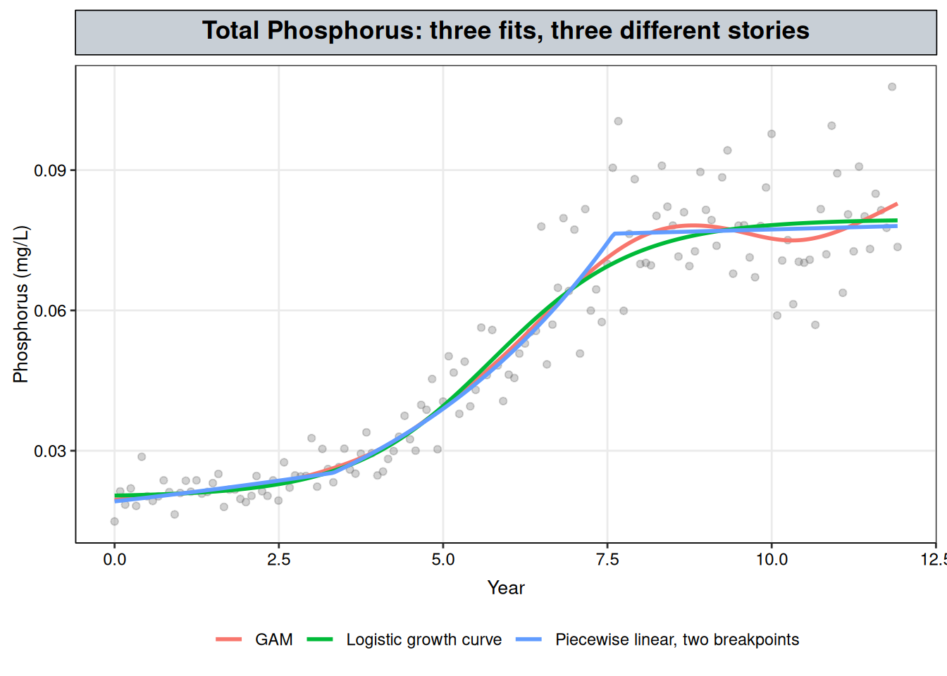
tp_grid <-data.frame(year_frac =seq(min(tp_wq$year_frac), max(tp_wq$year_frac), length.out =300))family_curves <-bind_rows(data.frame(model ="Logistic growth curve", year_frac = tp_grid$year_frac,fit =exp(predict(fit_logistic, newdata = tp_grid))),data.frame(model ="Piecewise linear, two breakpoints", year_frac = tp_grid$year_frac,fit =exp(predict(fit_piecewise, newdata = tp_grid))),data.frame(model ="GAM", year_frac = tp_grid$year_frac,fit =exp(as.numeric(predict(fit_tp_gam, newdata = tp_grid)))))ggplot() +geom_point(data = tp_wq, aes(year_frac, result), alpha =0.3, color ="grey40") +geom_line(data = family_curves, aes(year_frac, fit, color = model), linewidth =1) +labs(x ="Year", y ="Phosphorus (mg/L)", title ="Total Phosphorus: three fits, three different stories", color =NULL) + nlt_theme +theme(legend.position ="bottom")
Figure 1: Total Phosphorus with three fits on the log scale, back-transformed to mg/L: a logistic growth curve, a two-breakpoint piecewise linear regression and a GAM.
The three fits are close: their AICs span 2.0 units, which is too small to give preference to one model over another. Their curves overlap across most of the record (Figure 1).
They disagree on what happened. The logistic curve reports a ceiling of 0.079 mg/L (95% CI 0.076–0.083), which reads like a limit the concentration cannot pass. The piecewise model reports two breakpoints, at year 3.3 (95% CI 2.7–4.0) and year 7.6 (95% CI 7.2–8.0), which read like the dates of two events: something started, and something finished. Both sets of intervals are narrow. But each model fits the record as well as the other, and as well as a GAM that claims neither a ceiling nor any events. The intervals measure how precisely each parameter is located if that model is the right one. They are not evidence that a ceiling exists or that anything happened on those dates. A model that fits well yields small parameter variances whether or not other parameter sets, or other models, fit nearly as well, because the calculation assumes the fitted model is correct (Beven, 2006).
Different processes producing the same curve is known as equifinality (Beven, 2006), and it is the general problem with fitting a process-based curve to a record whose process is unknown. Each model’s parameters describe a story, and the data cannot tell the stories apart. Reporting a ceiling or a pair of event dates would report a process nobody established.
NoteHow this record was generated
The Total Phosphorus series on this site is synthetic, and it was generated from a logistic curve on the log scale: a floor of 0.02 mg/L, a ceiling of 0.08 mg/L, and a rise centred on year 5 (R/generate_synthetic_data.R). The logistic fit above recovers those values closely, with a floor of 0.02 mg/L, a ceiling of 0.079 mg/L and a midpoint at year 5.0.
Even here, where the logistic curve is the true one (in a synthetic record), the piecewise model and the GAM fit the record as well, so the record alone could not have confirmed the logistic form. A real monitoring record has no generator to check against, and a logistic curve would fit it just as convincingly whether or not any ceiling process existed.
4 Piecewise or GAM: different questions, not rivals
Inside the record, the three fits draw nearly the same curve. What separates them is what each one reports, and so which question it answers.
Which model answers which question
If the question is…
The estimand is…
Model that answers it
Is the record still rising?
The rate of change since the last shift
GAM, slope averaged over that stretch
How fast did it change over a period?
Average slope over that period
GAM averaged over the period, or a piecewise segment slope
A piecewise model reports dates. It estimates breakpoints with confidence intervals and a slope between each pair (Muggeo, 2008), and all of that assumes the breaks are real. Fit to a smooth rise like Total Phosphorus, it still returns breakpoints with narrow intervals, as above. They mark where the model joined two straight pieces, not when anything changed.
A GAM reports rates. It flags the stretches where the local slope differs from zero. Where a stretch begins depends on how much data surrounds it, how noisy that data is, and which interval is used (the simultaneous interval used here flags shorter stretches than a pointwise one would; Simpson, 2018). So a GAM supports “rising over roughly these years, at about this rate”, not “the change began in year X”.
For Total Phosphorus there is no known event, and the questions are whether the record is still rising and how fast it rose. Both are rates, so the GAM answers them without introducing dates the record cannot support.
5 Why Total Phosphorus is not forecast
Warning
Outside this site’s scope, shown on purpose. This site describes the observed record and does not forecast. This section makes one exception: it extends the logistic and GAM fits five years past the last sample to show what goes wrong when a model with no known process behind it is asked to forecast. Neither projection is a result to report.
The code below evaluates both fits on a grid that runs from the start of the record to five years past its end, with a 95% band around each. The GAM’s band comes from predict(). The logistic curve has no built-in equivalent, so its band is computed by the delta method, which propagates the uncertainty in its four fitted parameters through the curve. Both are fit on the log scale and converted back to mg/L.
record_end <-max(tp_wq$year_frac)proj_tp <-data.frame(year_frac =seq(min(tp_wq$year_frac), record_end +5, length.out =400))# logistic band by the delta method: numerical gradient of the curve with respect to its four parameterslogi_curve <-function(p) as.numeric(SSfpl(proj_tp$year_frac, p[1], p[2], p[3], p[4]))G <-sapply(seq_along(logi), function(i) { step <-replace(numeric(length(logi)), i, 1e-6) (logi_curve(logi + step) -logi_curve(logi - step)) /2e-6})logi_fit <-logi_curve(logi)logi_se <-sqrt(rowSums((G %*%vcov(fit_logistic)) * G))gam_proj <-predict(fit_tp_gam, newdata = proj_tp, se.fit =TRUE)proj_curves <-bind_rows(data.frame(model ="Logistic growth curve", year_frac = proj_tp$year_frac,fit = logi_fit, se = logi_se),data.frame(model ="GAM", year_frac = proj_tp$year_frac,fit =as.numeric(gam_proj$fit), se =as.numeric(gam_proj$se.fit))) |>mutate(est =exp(fit), lwr =exp(fit -1.96* se), upr =exp(fit +1.96* se),observed_range = year_frac <= record_end)proj_curves |>filter(year_frac ==max(year_frac)) |> dplyr::select(model, est, lwr, upr)
                  model        est        lwr        upr
1 Logistic growth curve 0.07947718 0.07573344 0.08340599
2                   GAM 0.12780873 0.05263390 0.31035267
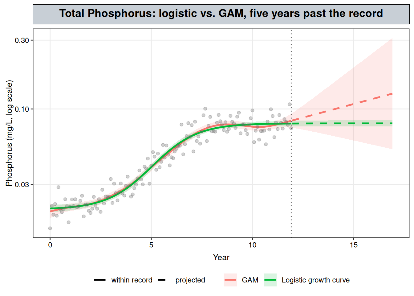
The printout is each model’s projected level five years after the last sample: est is the estimate in mg/L, and lwr and upr are the ends of its 95% band. Figure 2 shows the full curves.
ggplot(proj_curves, aes(year_frac)) +geom_ribbon(aes(ymin = lwr, ymax = upr, fill = model), alpha =0.15) +geom_line(aes(y = est, color = model, linetype = observed_range), linewidth =1) +geom_point(data = tp_wq, aes(year_frac, result), alpha =0.3, color ="grey40") +geom_vline(xintercept = record_end, linetype ="dotted", color ="grey30") +scale_y_log10() +# same colors as @fig-tp-familyscale_color_manual(values =c(GAM ="#F8766D", `Logistic growth curve`="#00BA38"), aesthetics =c("color", "fill")) +scale_linetype_manual(values =c(`TRUE`="solid", `FALSE`="dashed"), breaks =c(TRUE, FALSE),labels =c(`TRUE`="within record", `FALSE`="projected"), name =NULL) +labs(x ="Year", y ="Phosphorus (mg/L, log scale)", color =NULL, fill =NULL,title ="Total Phosphorus: logistic vs. GAM, five years past the record") + nlt_theme +theme(legend.position ="bottom")
Figure 2: The logistic and GAM fits to Total Phosphorus, extended five years past the last sample (dotted line), with pointwise 95% bands. Solid: within the record. Dashed: projected. Log scale.
Inside the record the two curves agree (Figure 2). Past it, they part ways:
The GAM breaks down. A penalized smooth is estimated from the data around each point, and past the last sample there is none. The thin plate smooth’s penalty acts on curvature, so with no data to bend it, the curve carries on roughly along its final slope on the log scale. The record ends on a small upturn, and the GAM carries it forward: from 0.083 mg/L (95% band 0.074–0.093) at the last sample to 0.128 mg/L (95% band 0.053–0.310) five years later. The widening band is the useful part of that output. It shows that the GAM has no information about those years.
The logistic curve stays flat by assumption. It projects 0.079 mg/L (95% band 0.076–0.083) five years out, the same to three decimal places as its 0.079 mg/L at the last sample. The narrow band does not come from the data showing that the plateau will hold. It comes from the formula, which cannot rise above its ceiling, and it covers uncertainty in the fitted parameters only, not any change in the process. A phosphorus plateau has no ceiling behind it in environmental chemistry. It reflects a balance between loading, flow, sediment release and uptake, and that balance shifts when land use, discharges or the monitoring program change. Reporting the ceiling as the future level asserts that the balance will hold, which nothing in the record shows.
Note
About this synthetic record. The logistic projection happens to be close to right here, because the generator is a logistic curve with a fixed ceiling. That is a property of how the data were made, not something the record could have shown.
Inside the record, the two fits agree, so for describing the record the GAM is enough and claims less. Outside the record, one model is unstable and the other is confident for a reason the data does not supply.
Tip
The gap between their projections is the cost of the mechanism assumption, made visible.
Neither projection is one this site would report; the next section describes the record instead, as a more supported approach, given the unknown process.
6 Reporting Total Phosphorus without claiming a process
The question still needs an answer. The GAM from Figure 1 gives one without choosing between the stories. It uses the same approach as the Total Copper case study: the local slope of the smooth and its confidence interval at each point mark each stretch of the record as rising, falling, or flat.
summary(fit_tp_gam)$s.table
                  edf   Ref.df        F p-value
s(year_frac) 6.790426 8.435197 262.1843       0
The printout is the test on the smooth term: edf is its effective degrees of freedom, a measure of how much the curve bends, and p-value tests whether it differs from a flat line.
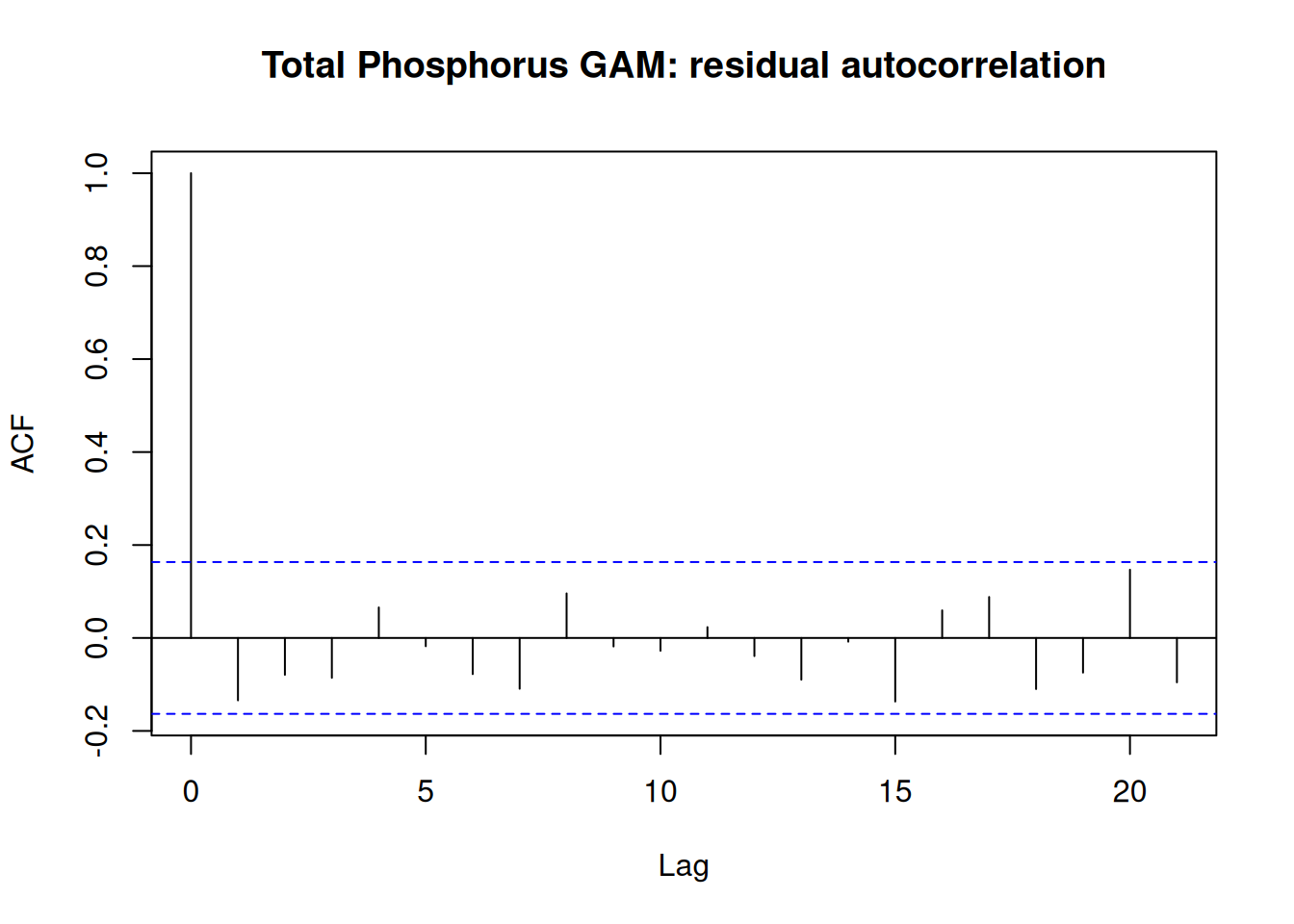
Every interval below rests on the residuals being independent. Generalized Additive Mixed Models showed that a regularly sampled record can fail that check without the fit giving any sign of it, so it comes first here (Figure 3).
acf(resid(fit_tp_gam), main ="Total Phosphorus GAM: residual autocorrelation")tp_box <-Box.test(resid(fit_tp_gam), lag =1, type ="Ljung-Box")tp_box
Figure 3: Residual autocorrelation of the Total Phosphorus GAM. The dashed lines are approximate 95% bounds for independent residuals.
Lag-1 autocorrelation is -0.13, and the Ljung-Box test finds no evidence against independence (\(p\) = 0.10). Unlike Dissolved Oxygen, this record needs no correlation structure, and the GAM’s intervals can be read as they stand.
The next chunk computes the local slope of the smooth at each point on a fine grid with gratia::derivatives() (Simpson, 2024), as in the GAM chapter, with a 95% simultaneous interval: one that covers the slope at all grid points at once, rather than each point on its own. A point is labelled rising or falling when its interval excludes zero, and flat otherwise. The printout gives the simultaneous critical value, which takes the place of 1.96, and the first and last years labelled rising.
set.seed(1) # the simultaneous critical value comes from posterior simulationtp_deriv <-derivatives( fit_tp_gam,select ="s(year_frac)",data = tp_grid,type ="central",interval ="simultaneous", # cover every grid point at once, not each point on its ownn_sim =10000# posterior draws used to find the critical value)pred <-predict(fit_tp_gam, newdata = tp_grid, se.fit =TRUE)tp_grid <- tp_grid |>mutate(fit =exp(pred$fit),# rising/falling only where the whole simultaneous interval clears zerotrend =case_when( tp_deriv$.lower_ci >0~"rising", tp_deriv$.upper_ci <0~"falling",TRUE~"flat" ) )rising <- tp_grid |>filter(trend =="rising")c(crit =unique(tp_deriv$.crit), rise_start =min(rising$year_frac), rise_end =max(rising$year_frac))
The slope is on the log scale, so it converts to a percent change per year. This chunk averages it over two stretches: the years labelled rising, and everything after them. An average over a stretch needs the covariance between the slopes at different dates, so it is computed from the model’s prediction matrix: the curve evaluated just either side of each grid point gives each slope as a linear combination of the coefficients, and averaging those combinations gives the stretch’s slope and its standard error. Each row of the printout is a slope in %/year with its 95% interval.
# finite-difference slope at each grid point, as a linear combination of the coefficientsh <-1e-3Xp_plus <-predict(fit_tp_gam, newdata =data.frame(year_frac = tp_grid$year_frac + h), type ="lpmatrix")Xp_minus <-predict(fit_tp_gam, newdata =data.frame(year_frac = tp_grid$year_frac - h), type ="lpmatrix")D <- (Xp_plus - Xp_minus) / (2* h)# average of the local slope over a stretch of the grid, with its SE, as %/yearperiod_slope <-function(rows) { a <-colMeans(D[rows, , drop =FALSE]) b <-sum(a *coef(fit_tp_gam)) s <-sqrt(drop(t(a) %*%vcov(fit_tp_gam) %*% a))100* (exp(c(slope = b, lower = b -1.96* s, upper = b +1.96* s)) -1)}rise_slope <-period_slope(tp_grid$trend =="rising")plateau_slope <-period_slope(tp_grid$year_frac >max(rising$year_frac))rbind(rise = rise_slope, since_rise = plateau_slope)
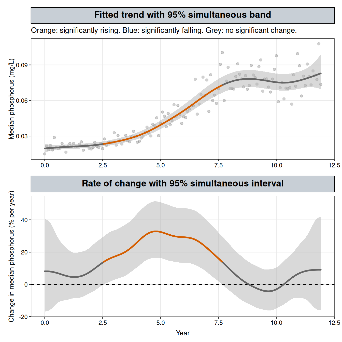
Figure 4 uses the same two-panel layout as the GAM and GAMM chapters (after Simpson, 2018, Figures 9 and 10). The top panel is the fitted median in mg/L with a 95% simultaneous band, built as in the GAM chapter: the critical value replacing 1.96 is the 95th percentile, across posterior draws of the coefficients, of the largest gap between the simulated and the fitted curve in standard errors. The bottom panel is the local slope from the chunk above, converted to percent per year, with its simultaneous interval.
# simultaneous band on the level (Simpson, 2018, Appendix 1), intercept included so it converts to mg/LXp <-predict(fit_tp_gam, newdata = tp_grid, type ="lpmatrix")se <-as.vector(pred$se.fit)set.seed(1) # the critical value comes from posterior simulationb_dev <- mgcv::rmvn(10000, mu =rep(0, length(coef(fit_tp_gam))), V =vcov(fit_tp_gam))crit_level <-unname(quantile(apply(abs((Xp %*%t(b_dev)) / se), 2, max), 0.95))tp_grid <- tp_grid |>mutate(# band built on the log scale, then exponentiatedlower_sim =exp(pred$fit - crit_level * se),upper_sim =exp(pred$fit + crit_level * se),# log-scale slope as % change per year in median phosphorus: (exp(slope) - 1) * 100pct = (exp(tp_deriv$.derivative) -1) *100,pct_lower = (exp(tp_deriv$.lower_ci) -1) *100,pct_upper = (exp(tp_deriv$.upper_ci) -1) *100 )# same colours as the GAM and GAMM chapterstrend_cols <-c(rising ="#D55E00", falling ="#0072B2", flat ="grey40")p_level <-ggplot(tp_grid, aes(year_frac)) +geom_point(data = tp_wq, aes(year_frac, result), alpha =0.3, color ="grey40") +geom_ribbon(aes(ymin = lower_sim, ymax = upper_sim), fill ="grey70", alpha =0.5) +geom_line(aes(y = fit, colour = trend, group =1), linewidth =1.1, lineend ="round") +scale_colour_manual(values = trend_cols) +labs(x =NULL, y ="Median phosphorus (mg/L)",title ="Fitted trend with 95% simultaneous band",subtitle ="Orange: significantly rising. Blue: significantly falling. Grey: no significant change.") + nlt_themep_rate <-ggplot(tp_grid, aes(year_frac)) +geom_ribbon(aes(ymin = pct_lower, ymax = pct_upper), fill ="grey70", alpha =0.5) +geom_hline(yintercept =0, linetype ="dashed") +geom_line(aes(y = pct, colour = trend, group =1), linewidth =1.1, lineend ="round") +scale_colour_manual(values = trend_cols) +labs(x ="Year", y ="Change in median phosphorus (% per year)",title ="Rate of change with 95% simultaneous interval") + nlt_themep_level / p_rate
Figure 4: Total Phosphorus GAM. Top: the fitted median with its 95% simultaneous band, coloured where the trend is significantly rising (orange) or falling (blue). Bottom: the rate of change, in percent per year, with its 95% simultaneous interval; a stretch is coloured where that interval excludes zero.
Both bands in Figure 4 are simultaneous, with critical values of 3.09 for the level and 3.21 for the slope, against 1.96 for a pointwise interval. The bottom panel is the evidence. The rate interval sits wholly above zero from about year 2.6 to year 7.7, and that stretch is coloured orange in both panels. The fastest rise in the fitted median is about 33% per year, near year 4.8. Outside that stretch the interval includes zero throughout. The shallow dip after year 9 and the upturn near the end of the record both show up in the fitted rate, but neither moves the interval clear of zero, and no stretch is coloured blue. The rate interval also widens toward both ends of the record, where fewer samples lie on one side of each date, so a slope there would have to be larger to count as significant.
The answer to the question. The GAM supports three statements, each with a different standing:
The record changed. The smooth term is significant (edf 6.8, \(p\) < 0.001). This is the formal test that the record is not flat, and it does not depend on choosing any period.
It rose from about year 2.6 to year 7.7, at an average of +24.9% per year (95% CI +22.9% to +27.0%). This averages the local slope over the stretch where it is significantly positive. Because that stretch was picked from the same fit, its interval excluding zero is built in. The number describes how fast the rise was and how precisely the record pins that down; it is not a separate test that a rise happened.
Since then, the evidence for further rise is weak. After year 7.7, no single date has a slope whose simultaneous interval clears zero. Averaged over that stretch, the slope is +3.1% per year (95% CI +0.01% to +6.2%), an interval that only just excludes zero. The average mixes three parts of the fitted curve: the end of the rise, which keeps tapering off for about a year; a shallow dip around years 9 to 10; and an upturn over the last year and a half of the record. The positive parts outweigh the dip, but none of the three is large enough at any single date to clear the wider simultaneous interval, and the GAM cannot separate the dip and the upturn from noise.
These are the statements the three fits agreed on, obtained without taking the logistic or piecewise story on board. Three cautions apply. “Flat” means the slope cannot be told apart from zero, not that it is shown to be zero. The start and end years of the rise are approximate: they mark where the simultaneous interval happens to cross zero on the grid, and a slope that changes gradually clears zero gradually. And the average after the rise depends on where that stretch begins. Here it begins where the interval on the slope stops clearing zero, which places the tapering end of the rise inside it. A later start would leave the taper out, but the upturn near the end would still pull the average up, and a start chosen after seeing the result would make the interval on that average harder to interpret.
If a specific event is suspected, such as a permit change or a new upstream discharge on a known date, that changes the situation: there is now a proposed process with a date attached. Piecewise Regression can test for a change in slope at that date, and Changepoint Detection can check whether the data independently places a break near it.
7 When a forecast is justified: decay after a source is removed
Warning
Outside this site’s scope, by design. This site describes the observed record and does not forecast. This section is the one case where a forecast is reported, because a known process supports carrying the fit past the last sample. The steps below show what that support has to include.
Total Phosphorus sits in the top-left cell of the table at the start of this chapter: no known process, and a question about the observed record. A plume after source removal sits in the opposite cell. After a contaminant source is removed from a site, the regulator’s question is how long a monitoring well will take to reach its cleanup goal. That question reaches past the record, so only a known process can answer it.
7.1 Why a process model is justified here
The period after removal has a known start, and one kind of process dominates: losses, with no new mass coming in. When those losses each remove roughly a fixed fraction of what is present, concentration falls by a constant fraction each year. That is first-order decay, \(C(t) = C_0 e^{-kt}\), which is a straight line on the log scale, so the model is the log-transform-then-OLS fit from Transformations. US EPA guidance on monitored natural attenuation calls the slope of log concentration against time at a single well the point decay rate constant, and uses it to estimate the time needed to reach a remediation goal at that location (Newell et al., 2002). It is a rate for that well, not for the plume as a whole, and it is not a biodegradation rate: it mostly reflects how quickly the source is being depleted, with contributions from sorption, dispersion and biodegradation. The example below assumes the source was removed completely. Newell et al. (2002) describe that as the rare case: most sites with organic contamination keep some residual source even after active remediation, and the rate then tracks how fast that residual source is depleting.
set.seed(7)# quarterly sampling for 10 years after source removal; first-order decay with multiplicative noiseplume <-data.frame(years_since_removal =seq(0, 10, by =0.25)) |>mutate(conc =1200*exp(-0.3* years_since_removal) *exp(rnorm(n(), sd =0.3)))fit_plume <-lm(log(conc) ~ years_since_removal, data = plume)k_point <--coef(fit_plume)[["years_since_removal"]]k_ci <--rev(confint(fit_plume)["years_since_removal", ])c(k = k_point, k_ci)
        k    97.5 %     2.5 %
0.3112359 0.2775728 0.3448990
The fitted rate is \(k\) = 0.311 per year (95% CI 0.278–0.345).
7.2 Check 1: does the record follow the process?
First-order decay predicts a straight line on the log scale. A GAM fit to the same data is free to bend, so if it does no better than the line, the record shows no curvature the process does not allow. The interval on \(k\) also assumes independent residuals, the check run for Total Phosphorus above.
fit_plume_gam <-gam(log(conc) ~s(years_since_removal), data = plume, method ="REML")plume_box <-Box.test(resid(fit_plume), lag =1, type ="Ljung-Box")c(AIC_line =AIC(fit_plume), AIC_gam =AIC(fit_plume_gam), ljung_box_p = plume_box$p.value)
The GAM does no better than the line (AIC 26.0 vs. 25.6), and the residuals show no lag-1 autocorrelation (Ljung-Box \(p\) = 0.50).
7.3 Check 2: does the early record predict the later one?
A model used to forecast should be tested on forecasting. Fitting the first five years and predicting the last five does that within the record. The same EPA guidance asks that monitoring be enough to determine both the attenuation rate and how that rate is changing with time (Newell et al., 2002), which is the question this check puts to the record.
21 of the 21 second-half samples fall inside the first-half fit’s 95% prediction interval, so the check passes. It should here, because the synthetic plume was generated from first-order decay at a constant rate.
7.4 The answer: time to the cleanup goal
cleanup_goal <-5# µg/Ltime_to_goal <- (coef(fit_plume)[[1]] -log(cleanup_goal)) / k_point# range from where the 95% confidence band on the fitted line crosses the goalproj <-data.frame(years_since_removal =seq(0, 30, by =0.01))band <-predict(fit_plume, newdata = proj, interval ="confidence")time_to_goal_range <-c( proj$years_since_removal[which(band[, "lwr"] <=log(cleanup_goal))[1]], proj$years_since_removal[which(band[, "upr"] <=log(cleanup_goal))[1]])c(time_to_goal = time_to_goal, time_to_goal_range)
time_to_goal
     18.0731      16.7700      19.7000
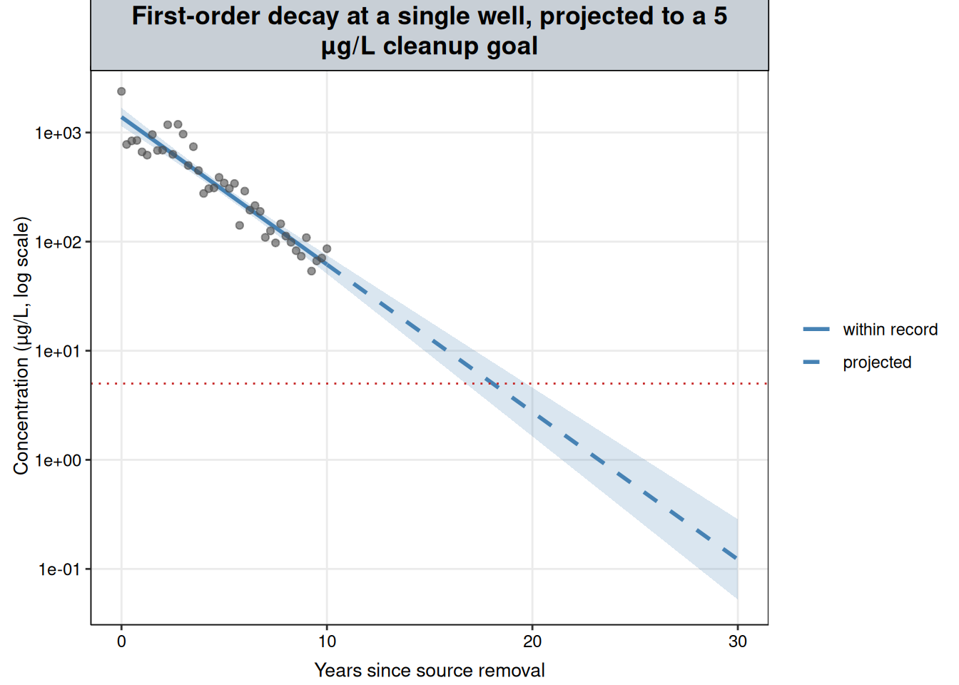
proj_df <- proj |>mutate(fit =exp(band[, "fit"]), lwr =exp(band[, "lwr"]), upr =exp(band[, "upr"]),observed_range = years_since_removal <=max(plume$years_since_removal))ggplot() +geom_ribbon(data = proj_df, aes(years_since_removal, ymin = lwr, ymax = upr), fill ="steelblue", alpha =0.2) +geom_line(data = proj_df, aes(years_since_removal, fit, linetype = observed_range), color ="steelblue", linewidth =1) +geom_point(data = plume, aes(years_since_removal, conc), alpha =0.6, color ="grey30") +geom_hline(yintercept = cleanup_goal, linetype ="dotted", color ="#C62828") +scale_y_log10() +scale_linetype_manual(values =c(`TRUE`="solid", `FALSE`="dashed"), breaks =c(TRUE, FALSE),labels =c(`TRUE`="within record", `FALSE`="projected"), name =NULL) +labs(x ="Years since source removal", y ="Concentration (µg/L, log scale)",title ="First-order decay at a single well, projected to a 5 µg/L cleanup goal") + nlt_theme +theme(legend.position ="right")
Figure 5: Synthetic plume record at a single well after source removal, with the first-order decay fit and its 95% confidence band, projected to the 5 µg/L cleanup goal (red dotted line). Solid: within the record. Dashed: projected. Log scale.
At the fitted rate (Figure 5), the well reaches 5 µg/L about 18.1 years after source removal, with the 95% confidence band crossing the goal between 16.8 and 19.7 years. Unlike the Total Phosphorus projection, this one is reportable, because the process says the decline continues after the last sample and both checks support it. The range covers uncertainty in the fitted line only, not a change in the process. The point decay calculation does not account for changes in attenuation processes, some of which can slow the apparent rate as concentrations fall (Newell et al., 2002), and forecast uncertainty grows with the length of the horizon (Kelly et al., 2013). The estimate should be updated as monitoring continues.
8 When a process-based model is justified
Total Phosphorus and the plume differ in a few specific ways. Those differences work as a checklist before fitting a model whose parameters claim a process:
What number does the decision need? A rate of change over a period, whether a record is still changing, or a time to reach a goal. This sets what the model has to produce.
Does the answer need to reach past the record? If not, a description of the record is usually enough, and a GAM gives one without claiming a process. If so, only a supported process can justify where the curve goes.
Is there a known event or starting point? Source removal starts the clock for a decay curve. Without one, a model’s timing parameters, such as breakpoints or a logistic midpoint, are fitted to the shape alone.
Does one process, or one kind of process, dominate? Losses after source removal do. Total Phosphorus’s mix of loading, flow, sediment release and uptake does not. Many overlapping influences of similar size point away from a single process-based curve.
Does the process predict something checkable, and does the record pass? For first-order decay: a straight line on the log scale, and an early-record rate that predicts the later record.
When these point to a known process, the process-based model is the stronger choice: its parameters answer the question directly, can be compared across sites, and, within the process’s limits, can be projected forward. When they do not, a GAM’s description of the record is the more defensible report.
9 Interpretation
A fit is not an explanation. A model is chosen by the question, by what is known about how the data arose, and by how far the answer has to reach, not by shape alone.
For Total Phosphorus, the process is unknown and the question is about the observed record. A logistic curve, a two-breakpoint piecewise model and a GAM fit it about equally well. The first two each tell a story, a ceiling or a pair of event dates, that the record cannot confirm, even though this synthetic record was in fact generated from a logistic curve. Projected past the record, the GAM becomes unstable and the logistic curve stays flat only because its formula requires it. With an unknown process and no need to forecast, the GAM is the more defensible model for this record. Its report is that the record changed (smooth term \(p\) < 0.001); that it rose from about year 2.6 to year 7.7 at an average of +24.9% per year (95% CI +22.9% to +27.0%); and that after year 7.7 no single date shows a significant slope, although the average over that stretch, +3.1% per year (95% CI +0.01% to +6.2%), only just excludes zero, from the tapering end of the rise and a small upturn near the end of the record that the GAM cannot separate from noise.
For the plume, a known process and a question that reaches past the record justify a first-order model. Its parameter answers the question directly, a cleanup date about 18.1 years after removal (16.8–19.7 years from the confidence band), and the record passes both the straight-line check and the split-record check.
Two things would change the Total Phosphorus choice: a documented event on a known date, which moves the record to Piecewise Regression with the break fixed at that date, or independent evidence for a process together with a question that reaches past the record.
The same reasoning applies across this site. Each method chapter matched a model to a shape, and Linear vs. Nonlinear Comparison checked that the flexibility was earned. The question, the data-generating process and how far the answer has to reach decide which of those models belongs in a report, and what its numbers can be taken to mean.
10 References
Beven, K. (2006). A manifesto for the equifinality thesis. Journal of Hydrology, 320(1–2), 18–36. https://doi.org/10.1016/j.jhydrol.2005.07.007
Hirsch, R.M., Alexander, R.B., and Smith, R.A. (1991). Selection of methods for the detection and estimation of trends in water quality. Water Resources Research, 27(5), 803–813.
Kelly (Letcher), R.A., Jakeman, A.J., et al. (2013). Selecting among five common modelling approaches for integrated environmental assessment and management. Environmental Modelling & Software, 47, 159–181.
Muggeo, V.M.R. (2008). segmented: An R package to fit regression models with broken-line relationships. R News, 8(1), 20–25.
Newell, C.J., Rifai, H.S., Wilson, J.T., Connor, J.A., Aziz, J.A., and Suarez, M.P. (2002). Calculation and Use of First-Order Rate Constants for Monitored Natural Attenuation Studies. Ground Water Issue, EPA/540/S-02/500. U.S. Environmental Protection Agency.
Simpson, G.L. (2018). Modelling palaeoecological time series using generalised additive models. Frontiers in Ecology and Evolution, 6, 149.
Simpson, G.L. (2024). gratia: An R package for exploring generalized additive models. Journal of Open Source Software, 9(104), 6962. https://doi.org/10.21105/joss.06962. Version 0.11.2 used.
Wood, S.N. (2017). Generalized Additive Models: An Introduction with R, Second Edition. CRC Press.